Robust correlation analyses: false positive and power validation using a new open source matlab toolbox

Abstract

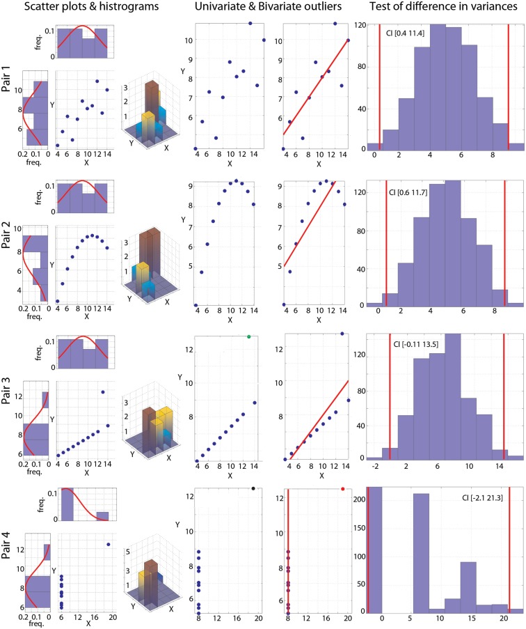
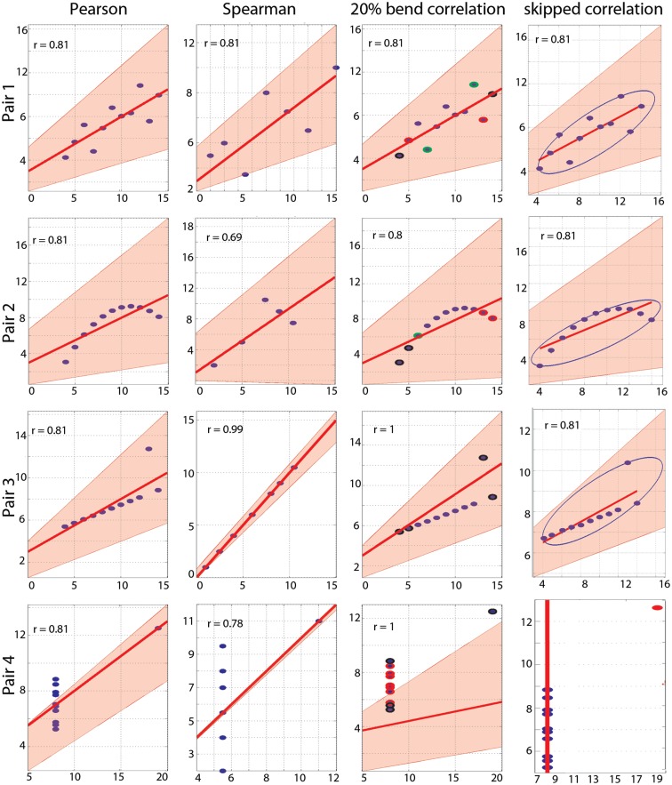
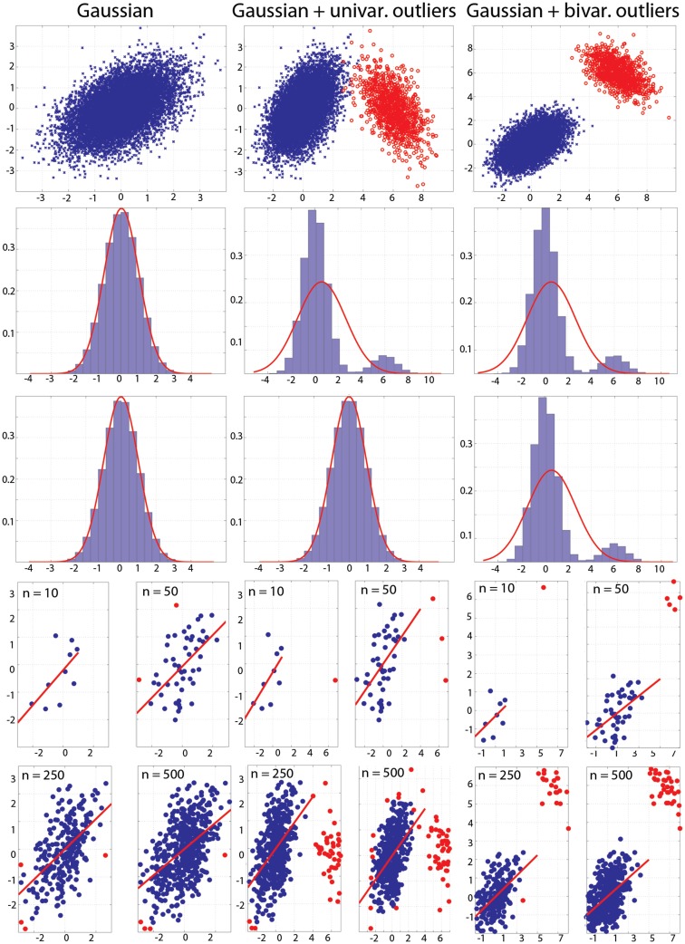
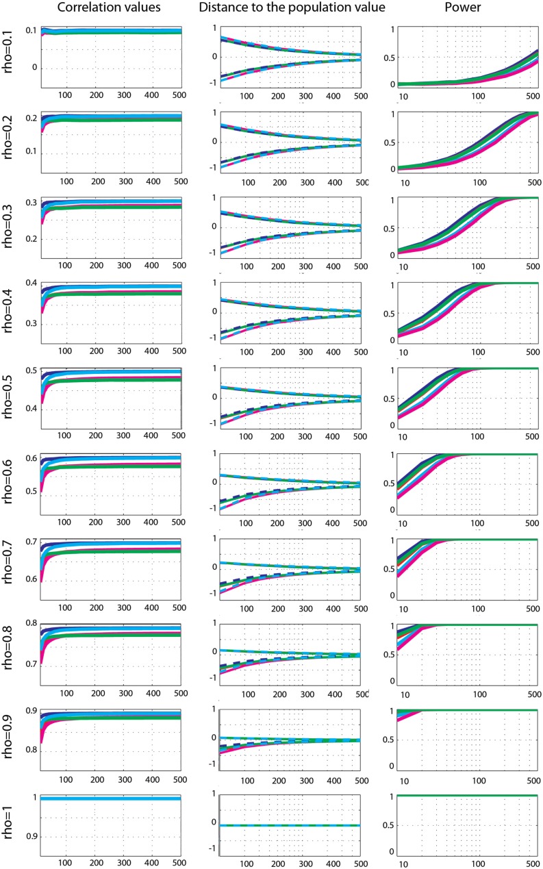
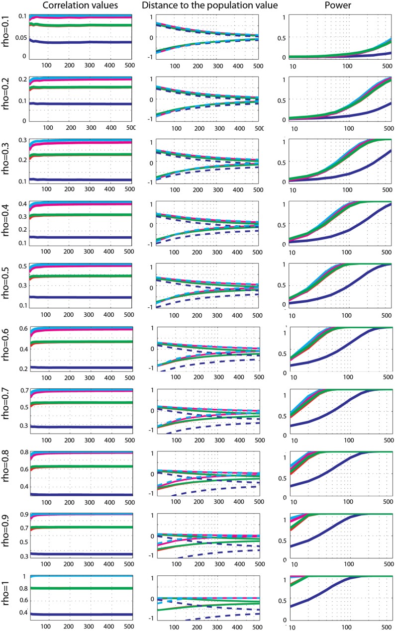
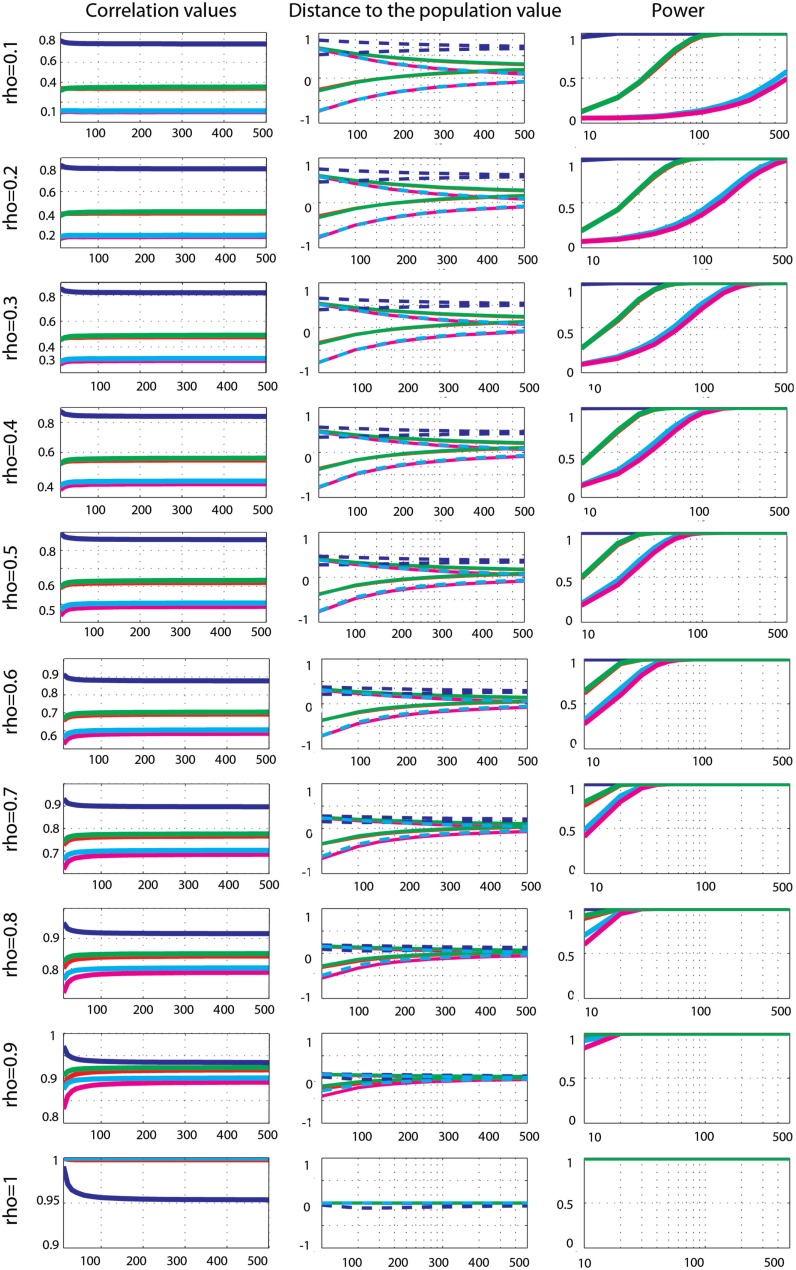
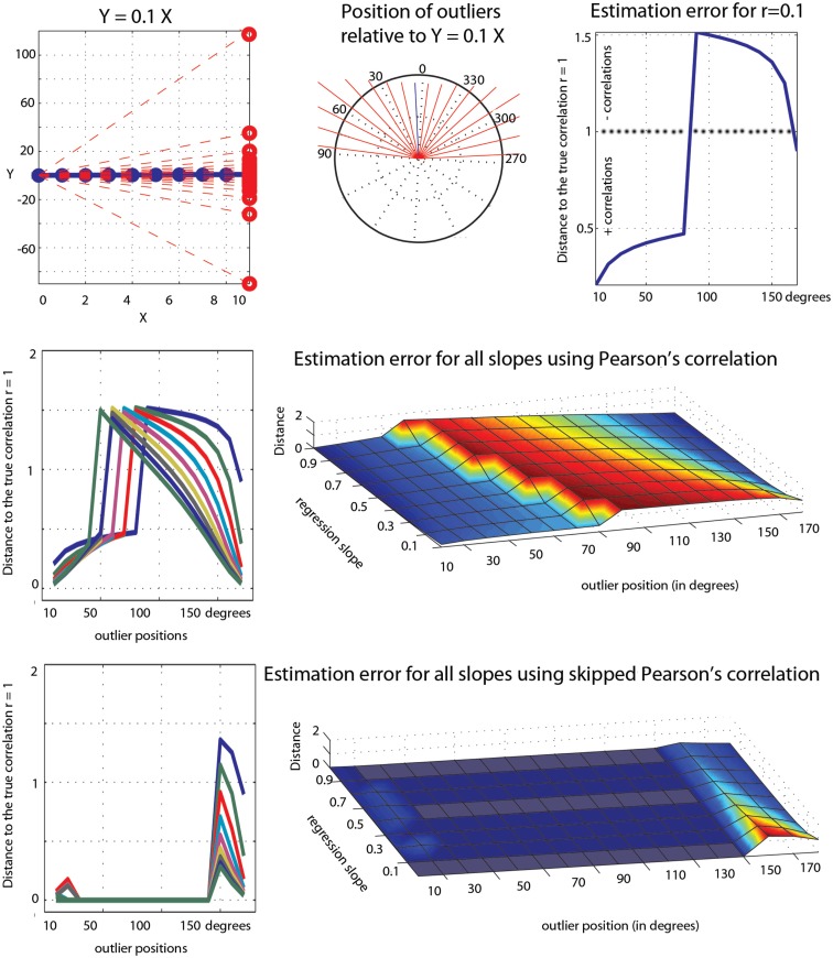
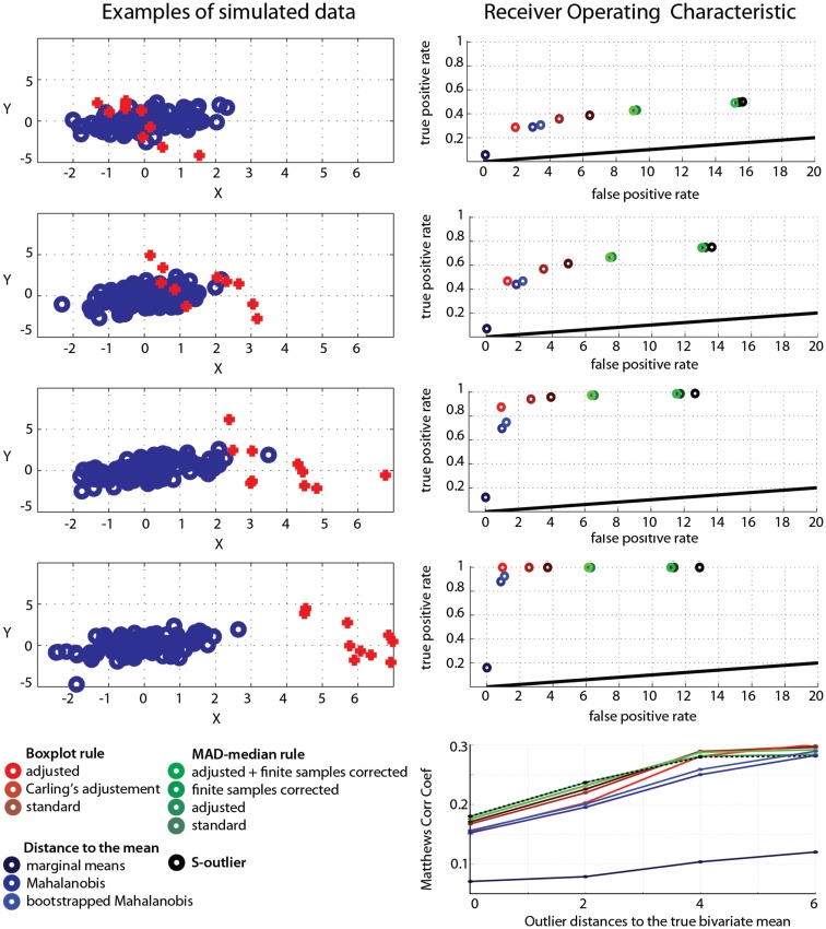
Pearson's correlation measures the strength of the association between two variables. The technique is, however, restricted to linear associations and is overly sensitive to outliers. Indeed, a single outlier can result in a highly inaccurate summary of the data. Yet, it remains the most commonly used measure of association in psychology research. Here we describe a free Matlab((R)) based toolbox (http://sourceforge.net/projects/robustcorrtool/) that computes robust measures of association between two or more random variables: the percentage-bend correlation and skipped-correlations. After illustrating how to use the toolbox, we show that robust methods, where outliers are down weighted or removed and accounted for in significance testing, provide better estimates of the true association with accurate false positive control and without loss of power. The different correlation methods were tested with normal data and normal data contaminated with marginal or bivariate outliers. We report estimates of effect size, false positive rate and power, and advise on which technique to use depending on the data at hand.

Keywords: MATLAB; correlation; outliers; power; robust statistics.

Figure 1

Visualization of the Anscombe’s quartet. Each pair is illustrated by a scatter plot and with univariate and bivariate histograms (left column). Outliers detected using the box-plot rule are plotted in the two middle columns: column 2 shows univariate outliers in Y (green) or in X and Y (black); column 3 shows bivariate outliers (red), with the best line fitted to the remaining points. Histograms (right column) show the bootstrapped variance differences. Vertical red lines indicate 95% CIs.

Figure 2

Correlation results. From left to right are illustrated Pearson’s, Spearman’s, 20% bend, and Pearson’s skipped-correlations with the 95% bootstrapped CIs as pink shaded areas. The scale for Spearman’s correlations differs from the others because ranked data are plotted. For the 20% bend correlation, red indicates data bent in X, green in Y and black in both. No skipped correlation is returned for pair 4.

Figure 3

Populations used in the simulations. Top: populations with effect sizes of 0.5. Middle: marginal histograms for these populations. Bottom: examples of draws with sample sizes n = 10, 50, 250, and 500. Red dots mark bivariate outliers identified using the box-plot rule on project data.

Figure 4

Effect sizes and false positive error rates for Gaussian data with zero-correlation. From left to right are displayed: the mean correlation values; the 99.99% CIs (i.e., corrected for the 14 sample sizes) of the distance to the zero-correlation in the simulated Gaussian population; the false positive rate for Pearsons’ (blue), skipped Pearson’s (cyan), Spearman’s (red), skipped Spearman’s (magenta), and 20% bend (green) correlations for each type of simulation (Gaussian only, with univariate outliers, and with bivariate outliers). The Y-axis scales are different for data with bivariate outliers.

Figure 5

Effect sizes and power for Gaussian data. From left to right are displayed: the mean correlation values; the 99.99% CIs (i.e., corrected for the 14 sample sizes) of the distance to the correlation in the simulated Gaussian population; the power for Pearson’s (blue), skipped Pearson’s (cyan), Spearman’s (red), skipped Spearman’s (magenta), and 20% bend (green) correlations for each effect size (from top r = 0.1 to bottom r = 1).

Figure 6

Effect sizes and power for Gaussian data contaminated by 10% of marginal outliers. From left to right are displayed: the mean correlation values; the 99.99% CIs (i.e., corrected for the 14 sample sizes) of the distance to the correlation in the simulated Gaussian population contaminated by univariate outliers; the power for Pearson’s (blue), skipped Pearson’s (cyan), Spearman’s (red), skipped Spearman’s (magenta), and 20% bend (green) correlations for each effect size (from top r = 0.1 to bottom r = 1). In column one, the scales of the mean correlation values differ.

Figure 7

Effect sizes and power for Gaussian data contaminated by 10% of bivariate outliers. From left to right are displayed: the mean correlation values; the 99.99% CIs (i.e., corrected for the 14 sample sizes) of the distance to the correlation in the simulated Gaussian population contaminated by bivariate outliers; the power for Pearson’s (blue), skipped Pearson’s (cyan), Spearman’s (red), skipped Spearman’s (magenta), and 20% bend (green) correlations for each effect size (from top r = 0.1 to bottom r = 1). In column one, the scales of the mean correlation values differ.

Figure 8

Illustration of the effect of a single outlier among 10 data points on Pearson’s correlation. At the top is illustrated the outlier values (red circles in the left plot), their positions in the bivariate space (the end of each red line in the polar plot) relative to the regression line Y = 0.1X, and the error in Pearson’s estimates (1 – observed correlation). The middle row shows similar results for all slopes (from 0.1 to 0.9). The bottom row shows the results from the skipped correlation.

Figure A1

Operating characteristics of outlier detection methods. The left column illustrates the data generation process: each row shows different types of outliers, identified in red, and created by changing the amount of shift along the X direction. The right column shows the false positive rate (1-specificity) as a function of the true positive rate (sensitivity) for each method. Bottom right show the Matthews correlation coefficients. Red to brown: box-plot results; light green to dark green: MAD-median rule results; black: the S-outlier results; light to dark blue: deviations from the mean(s) results.

References

1. Barnett V., Lewis T. (1994). Ouliers in Statistical Data. Chichester: Wiley
1. Bakli P., Brunak S., Chauvin Y., Anderson C. A., Nielsen H. (2000). Assessing the accuracy of prediction algorithms for classification: an overview. Bioinformatics 16, 412–42410.1093/bioinformatics/16.5.412 - DOI - PubMed
1. Anscombe F. J. (1973). Graphs in statistical analysis. Am. Stat. 27, 17–2110.1080/00031305.1973.10478966 - DOI
1. Carling K. (2000). Resistant outlier rules and the non-Gaussian case. Stat. Data Anal. 33, 249–25810.1016/S0167-9473(99)00057-2 - DOI
1. Erceg-Hurn D. M., Mirosevich V. M. (2008). Modern robust statistical methods: an easy way to maximize the accuracy and power of your research. Am. Psychol. 63, 591.10.1037/0003-066X.63.7.591 - DOI - PubMed
LinkOut - more resources