A virtual retina for studying population coding

Abstract

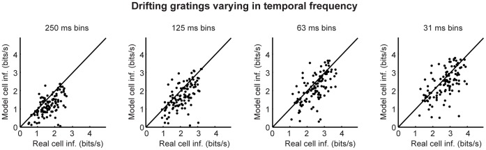
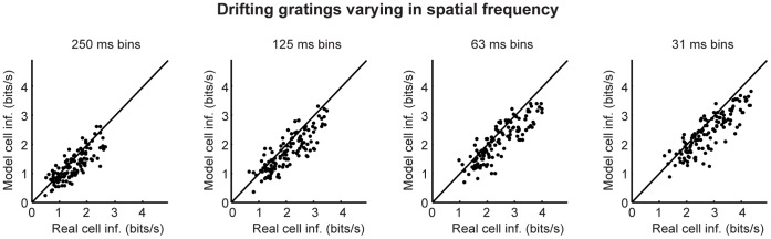
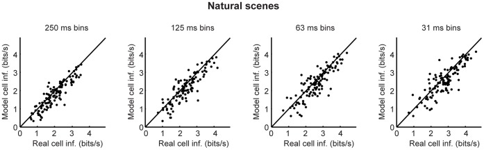
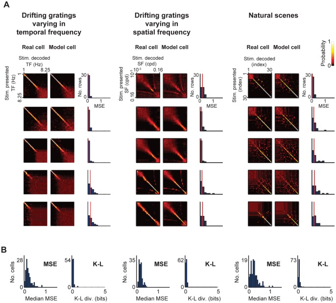
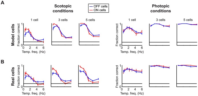
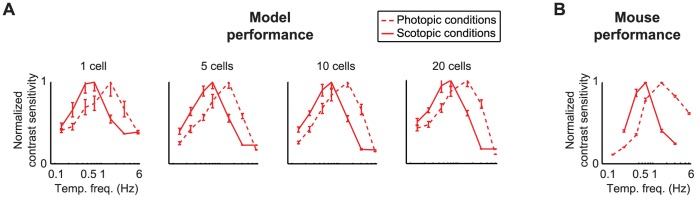
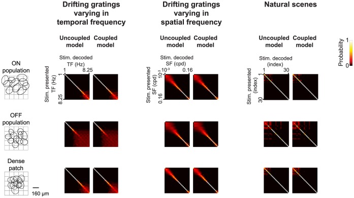
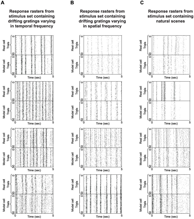
At every level of the visual system - from retina to cortex - information is encoded in the activity of large populations of cells. The populations are not uniform, but contain many different types of cells, each with its own sensitivities to visual stimuli. Understanding the roles of the cell types and how they work together to form collective representations has been a long-standing goal. This goal, though, has been difficult to advance, and, to a large extent, the reason is data limitation. Large numbers of stimulus/response relationships need to be explored, and obtaining enough data to examine even a fraction of them requires a great deal of experiments and animals. Here we describe a tool for addressing this, specifically, at the level of the retina. The tool is a data-driven model of retinal input/output relationships that is effective on a broad range of stimuli - essentially, a virtual retina. The results show that it is highly reliable: (1) the model cells carry the same amount of information as their real cell counterparts, (2) the quality of the information is the same - that is, the posterior stimulus distributions produced by the model cells closely match those of their real cell counterparts, and (3) the model cells are able to make very reliable predictions about the functions of the different retinal output cell types, as measured using Bayesian decoding (electrophysiology) and optomotor performance (behavior). In sum, we present a new tool for studying population coding and test it experimentally. It provides a way to rapidly probe the actions of different cell classes and develop testable predictions. The overall aim is to build constrained theories about population coding and keep the number of experiments and animals to a minimum.

Figure 1. The amount of information carried by the model cells closely matched that of their real cell counterparts, when the stimulus set consisted of drifting gratings that varied in temporal frequency.

The mutual information between each model cell’s responses and the stimuli was calculated and plotted against the mutual information between its corresponding real cell’s responses and the stimuli. Bin sizes ranged from 250 ms to 31 ms; n = 109 cells; stimulus entropy was 4.9 bits (30 one-second movie snippets). Note that there is scatter both above and below the line because of data limitation.

Figure 2. The amount of information carried by the model cells closely matched that of their real cell counterparts, when the stimulus set consisted of drifting gratings that varied in spatial frequency.

As in Fig. 1, the mutual information between each model cell’s responses and the stimuli was calculated and plotted against the mutual information between its corresponding real cell’s responses and the stimuli. Bin sizes ranged from 250 ms to 31 ms; n = 120 cells; stimulus entropy was 4.9 bits (30 one-second movie snippets). Note that there is scatter both above and below the line because of data limitation.

Figure 3. The amount of information carried by the model cells closely matched that of their real cell counterparts, when the stimulus set consisted of natural scene movies.

As in Figs. 1 and 2, the mutual information between each model cell’s responses and the stimuli was calculated and plotted against the mutual information between its corresponding real cell’s responses and the stimuli. Bin sizes ranged from 250 ms to 31 ms; n = 113 cells; stimulus entropy was 4.9 bits (30 one-second movie snippets). Note that there is scatter both above and below the line because of data limitation.

Figure 4. The posterior stimulus distributions of the model cells closely matched those of their real cell counterparts.

(A) Pairs of matrices for each cell. The matrix on the left gives the posterior stimulus distributions for the real cell’s responses; the matrix on the right gives the same for the model cell’s responses. The histogram next to the pair gives a measure of the distance between them. Briefly, for each row, we computed the mean squared error (MSE) between the model’s posterior and the real cell’s posterior and then normalized it by dividing it by the MSE between the real cell’s posterior and a randomly shuffled posterior. A value of 0 indicates that the two rows are identical. A value of 1 indicates that they are as different as two randomly shuffled rows. Because of data limitation, occasional cells showed values higher than 1. The vertical red line indicates the median value of the histogram, the MSE α value. (B) Histogram of the MSE α values for all cells in the data set, and histogram of the K-L α values for all cells in the data set (n = 109, 120 and 113 cells for the stimuli, respectively). As shown in these histograms, most of the distances are low. For the MSE, the median α value is 0.21. As mentioned above, 0 indicates a perfect match between model and real responses, and 1 indicates correspondence no better than chance. For the K-L divergence, the median α value is 0.18. As a reference, 0 indicates a perfect match between model and real responses, and 4.9 bits (the stimulus entropy) indicates a poor match – this would be the K-L divergence between perfect decoding by a real cell and random decoding by a model cell. The complete set of matrices for the data set are provided in Figs. S1, S2, S3.

Figure 5. The model was able to make reliable predictions about the behavior of the real cell classes.

Each plot shows the “fraction correct” as a function of temporal frequency for ON cells (red) and OFF cells (blue). Top left, the model indicates that ON cells are better at distinguishing among low temporal frequencies than OFF cells under scotopic conditions, whereas OFF cells are better at distinguishing among high temporal frequencies. Bottom left, the real cells indicate the same. Top, looking across scotopic and photopic conditions, the model indicates that these differences only occur under scotopic conditions. Bottom, looking across scotopic and photopic conditions, the real cells indicate the same. Top, looking across the two conditions , the model shows that ON and OFF cells perform well only for a narrow range of frequencies under scotopic conditions, but over a broad range under photopic conditions. Bottom, looking across the two conditions, this prediction held for the real cells as well. Predictions were made with increasing numbers of cells until there was indication of performance saturation. Error bars are SEM. The horizontal black line corresponds to performance at chance (7 stimuli, 1/7 correct).

Figure 6. The model predicted the shift in optomotor performance.

Each plot shows normalized contrast sensitivity under photopic and scotopic light conditions. (A) The model predicts a shift toward higher temporal frequencies as the animal moves from scotopic to photopic conditions, with the peak shifting from 0.7 Hz to 1.5 Hz. The prediction was robust from 1 cell to saturation (20 cells). (B) The animals’ behavioral performance shifted to higher temporal frequencies, as predicted (n = 5 animals). Error bars are SEM.

Figure 7. Posterior stimulus distributions generated using models that included correlations among the ganglion cells and models that treated the ganglion cells as independent.

The posterior stimulus distributions (matrices) were calculated using three populations of cells: a patch of transient ON cells (n = 10 cells), a patch of transient OFF cells (n = 11 cells), and a patch that included all the cells recorded in a local region of the retina (n = 12 cells). For each population, models were built without correlations (left) and with correlations (right) included. Distances between coupled and uncoupled posteriors were very low: MSE α values were below 0.05, and K-L α values were below 0.1 bits. To avoid data limitation, response distributions for the population were taken directly from the analytical form of the model, as in , .

Figure 8. Response rasters for the first 12 cells shown in Fig. 4.

Fig. 4 shows real and model cell performance using three sets of stimuli. Here we show rasters of the underlying responses. A. Rasters for the responses to the drifting gratings that varied in temporal frequency. The stimulus is a continuous stream of drifting gratings with uniform gray fields interleaved (grating stimuli are 1 s; gray fields are 0.33 s). 5 s of a 41 s stimulus are shown (repeated 50 times). Note that each cell is viewing a different location in the movie. B. Rasters for the responses to the drifting gratings that varied in spatial frequency. As above, the stimulus is a continuous stream of drifting gratings with uniform gray fields interleaved (grating stimuli are 1 s, gray fields are 0.33 s). Each cell is viewing a different location of the stimulus. C. Rasters for the responses to the natural scene movies. The stimulus is a continuous stream of natural movies with uniform gray fields interleaved (natural movie snippets are 1 s long, gray fields are 0.33 s). Note again that each cell is viewing a different location in the movie: this is most notable in the rasters for the natural scene snippets, since these are not periodic stimuli.

References

1. Smith DV, John SJ, Boughter JD (2000) Neuronal cell types and taste quality coding. Physiol Behav 69: 77–85. - PubMed
1. Di Lorenzo PM (2000) The neural code for taste in the brain stem: response profiles. Physiol Behav 69: 87–96. - PubMed
1. Laurent G (2002) Olfactory network dynamics and the coding of multidimensional signals. Nat Rev Neurosci 3: 884–895. - PubMed
1. Konishi M (2003) Coding of auditory space. Annu Rev Neurosci 26: 31–55. - PubMed
1. Field GD, Chichilnisky EJ (2007) Information processing in the primate retina: circuitry and coding. Annu Rev Neurosci 30: 1–30. - PubMed
Publication types
LinkOut - more resources