A fast least-squares algorithm for population inference

Abstract

Background: Population inference is an important problem in genetics used to remove population stratification in genome-wide association studies and to detect migration patterns or shared ancestry. An individual's genotype can be modeled as a probabilistic function of ancestral population memberships, Q, and the allele frequencies in those populations, P. The parameters, P and Q, of this binomial likelihood model can be inferred using slow sampling methods such as Markov Chain Monte Carlo methods or faster gradient based approaches such as sequential quadratic programming. This paper proposes a least-squares simplification of the binomial likelihood model motivated by a Euclidean interpretation of the genotype feature space. This results in a faster algorithm that easily incorporates the degree of admixture within the sample of individuals and improves estimates without requiring trial-and-error tuning.

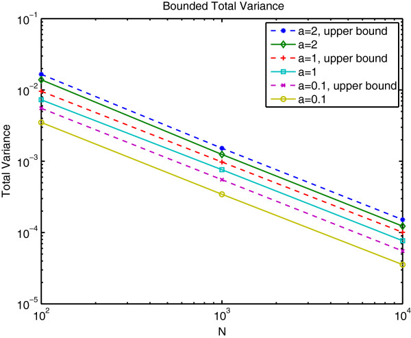
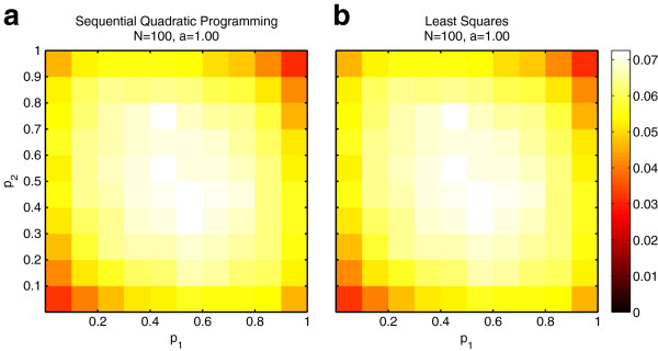
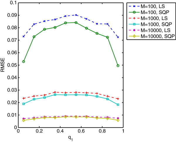
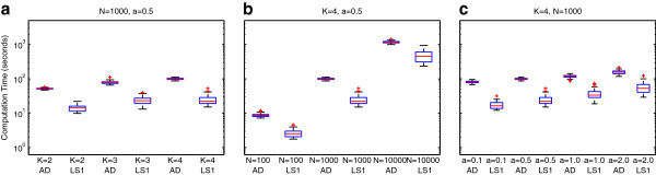
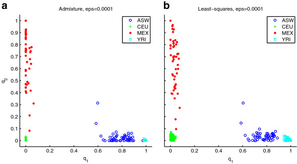
Results: We show that the expected value of the least-squares solution across all possible genotype datasets is equal to the true solution when part of the problem has been solved, and that the variance of the solution approaches zero as its size increases. The Least-squares algorithm performs nearly as well as Admixture for these theoretical scenarios. We compare least-squares, Admixture, and FRAPPE for a variety of problem sizes and difficulties. For particularly hard problems with a large number of populations, small number of samples, or greater degree of admixture, least-squares performs better than the other methods. On simulated mixtures of real population allele frequencies from the HapMap project, Admixture estimates sparsely mixed individuals better than Least-squares. The least-squares approach, however, performs within 1.5% of the Admixture error. On individual genotypes from the HapMap project, Admixture and least-squares perform qualitatively similarly and within 1.2% of each other. Significantly, the least-squares approach nearly always converges 1.5- to 6-times faster.

Conclusions: The computational advantage of the least-squares approach along with its good estimation performance warrants further research, especially for very large datasets. As problem sizes increase, the difference in estimation performance between all algorithms decreases. In addition, when prior information is known, the least-squares approach easily incorporates the expected degree of admixture to improve the estimate.

Figure 1

Bound on total variance. Solid and dashed lines correspond to the empirical estimate of the total variance and the upper bound for total variance, respectively.

Figure 2

Precision of best-case scenario for estimating P. Root mean squared error for different values of p using (a) Admixture’s Sequential Quadratic Programming or (b) the least-squares approximation.

Figure 3

Precision of best-case scenario for estimating Q. Solid and dashed lines correspond to Admixture’s Sequential Quadratic Programming optimization and the least-squares approximation, respectively.

Figure 4

Computational timing comparison. Box plots show the median (red line) and inter-quartile range (blue box) for computation time on a logarithmic scale using (a) N=1000, α=0.5, and varying K; (b) K=4, α=0.5, and varying N; and (c) K=4, N=1000, and varying α.

Figure 5

Comparison on HapMap Phase 3 dataset. Inferred population membership proportions using (a) Admixture and (b) least-squares with α=1. Each point represents a different individual among the four populations: ASW, CEU, MEX, and YRI. The axes represent the proportion of each individual’s genome originating from each inferred population. The proportion belonging to the third inferred population is given by q₃ = 1 – q₁ – q₂.

Figure 6

First-order approximation for slope of log-likelihood of m. Solid and dashed lines correspond to the true and approximated slope, respectively. The red, green, and blue lines correspond to g = 0, g = 1, and g = 2, respectively.

Figure 7

First-order approximation for slope of log-likelihood of q. Solid and dashed lines correspond to the true and approximated slope, respectively, for K = 2. The blue, green, red, and orange lines correspond to α = 0.1, α = 0.5, α = 1, and α = 2, respectively.