An electrophysiological validation of stochastic DCM for fMRI

Abstract

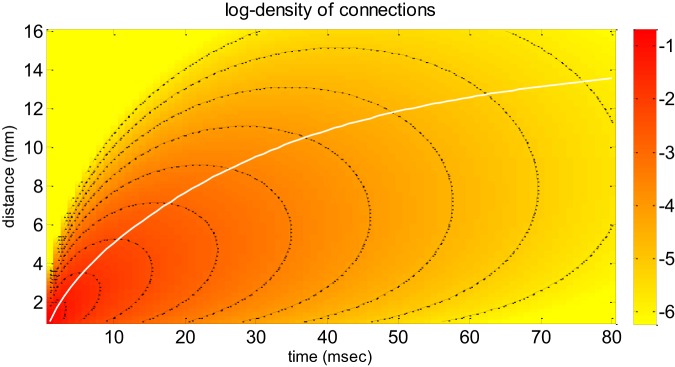
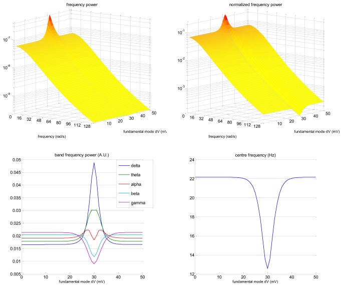
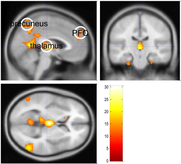
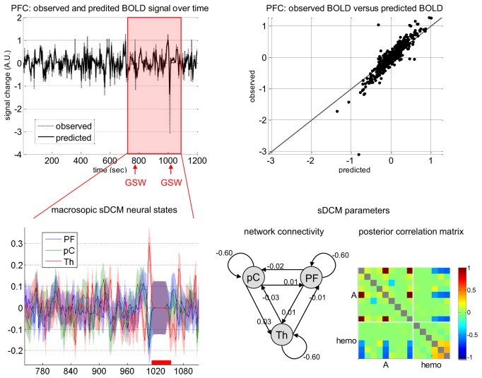
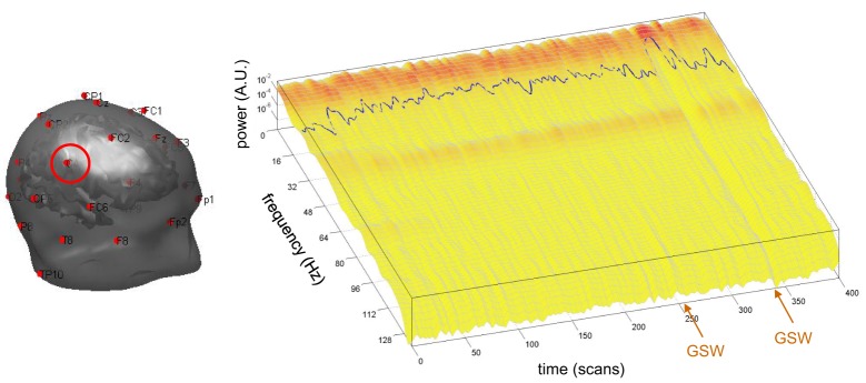
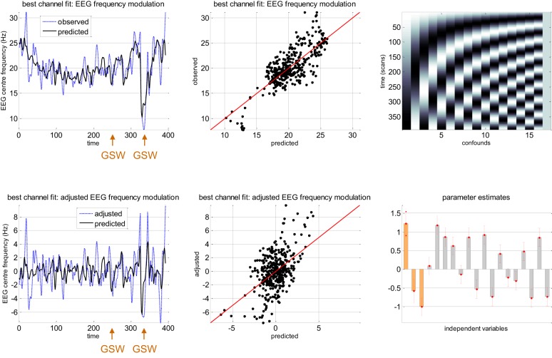
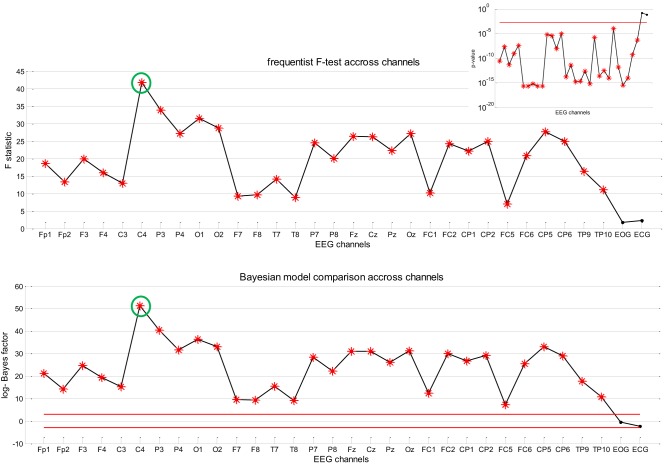
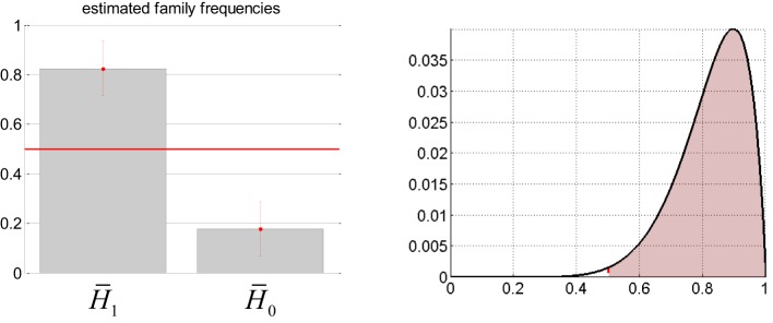
In this note, we assess the predictive validity of stochastic dynamic causal modeling (sDCM) of functional magnetic resonance imaging (fMRI) data, in terms of its ability to explain changes in the frequency spectrum of concurrently acquired electroencephalography (EEG) signal. We first revisit the heuristic model proposed in Kilner et al. (2005), which suggests that fMRI activation is associated with a frequency modulation of the EEG signal (rather than an amplitude modulation within frequency bands). We propose a quantitative derivation of the underlying idea, based upon a neural field formulation of cortical activity. In brief, dense lateral connections induce a separation of time scales, whereby fast (and high spatial frequency) modes are enslaved by slow (low spatial frequency) modes. This slaving effect is such that the frequency spectrum of fast modes (which dominate EEG signals) is controlled by the amplitude of slow modes (which dominate fMRI signals). We then use conjoint empirical EEG-fMRI data-acquired in epilepsy patients-to demonstrate the electrophysiological underpinning of neural fluctuations inferred from sDCM for fMRI.

Keywords: EEG; dynamic causal modeling; effective connectivity; fMRI; neural field; neural noise; separation of time scales.

Figure 1

Neural field model: the dispersive propagator. This figure depicts the dispersive propagator of Equation (4) as a function of both time (x-axis) and distance (y-axis), in terms of the density 2πrG(r, t) of synaptic connections that are reached by an action potential emitted at r = t = 0 (on a logarithmic scale). Note that the 2πr scaling arises because of radial symmetry in 2D (Bojak and Liley, 2010). The white line shows the average distance, at which activity is propagated as a function of time. The black lines are contour lines of the connection density. These can be used to eyeball how fast the density attenuates (e.g., along the average distance path).

Figure 2

Neural field model: EEG frequency modulation. This figure shows the effect of changes in the mean membrane depolarization fundamental eigenmode z⁽⁰⁾₁ on the frequency content of the EEG signal. Upper-left: EEG frequency spectrum P(ω) (z-axis) as a function of frequency ω (x-axis) and eigenmode amplitude z⁽⁰⁾₁ (y-axis). Upper-right: Normalized frequency spectrum $\overline{\text{P}}(\omega )$ (cf. Equation 10, same format). Lower-left: Magnitude of standard EEG frequency bands (y-axis; blue: delta, green: theta, red: alpha, magenta: beta, violet: gamma) as a function of the eigenmode amplitude z⁽⁰⁾₁ (x-axis). Lower-right: Centre frequency $\overline{\omega }$ (y-axis) as a function of the eigenmode amplitude z⁽⁰⁾₁ (x-axis). Note that here, the action potential firing threshold χ is 30 mV.

Figure 3

Absence seizure analysis: regions of interest. This figure summarizes the standard SPM activation results of a single epileptic patient with (petit mal) absence seizure (the same subject as in Figure 1). Significant (whole brain FWE-corrected, p < 0.05) positive and negative GSW-related BOLD responses were identified by means of an F-contrast on the GSW regressors. The color bar indicates the range of displayed F values.

Figure 4

Absence seizure analysis: sDCM analysis. This figure summarizes the sDCM analysis of a single subject fMRI data (same patient as in Figure 1). Upper-left: Time series of the observed and fitted BOLD signal in prefrontal cortex (PFC) as a function of time. The red shaded area indicates peri-GSW activity. Upper-right: Observed (y-axis) versus fitted (x-axis) BOLD signal in PFC. Lower-left: Macroscopic sDCM neural states in the three regions of interest (PF, prefrontal cortex; pC, precuneus; Th, thalamus) during peri-GSW activity, as a function of time. The red bar indicates strong head motion, which was modeled using scan-nulling regressors (see main text). Lower-right: sDCM conditional density on model parameters (left: first-order moment and ensuing network connectivity, right: posterior correlation matrix). Note: identifiability issues between pairs of parameters manifest as high posterior correlations.

Figure 5

Absence seizure analysis: derivation of the EEG frequency modulation. This figure depicts the extraction of the EEG center frequency in a single subject (same patient as in Figure 1). Left: The EEG set-up used during the recording session is shown superimposed on the brain and skin surfaces (sensor C4 is highlighted). Right: Normalized square root power of windowed Fourier transform (z-axis) of the EEG traces of sensor C4 (x-axis: scanning time, y-axis: instantaneous frequency). The blue line shows the center frequency $\overline{\omega }$ as a function of scanning time t (cf. Equation 10 in the main text).

Figure 6

Absence seizure analysis: EEG results (1). This figure summarizes the results of the analysis on the EEG frequency modulation in a single subject (same patient as in Figure 5) at channel C4. Upper-left: Observed (blue dashed line) and predicted (black plain line) frequency modulation (y-axis) of the best EEG channel (C4) as a function of scanning time (x-axis). For this patient, the two GSW episodes are indicated by the orange arrows. Upper-middle: Observed (y-axis) versus predicted (x-axis) frequency modulation for EEG channel C4. Upper-right: Matrix of confounds X₀ included in the analysis (slow drifts). Lower-left: Observed (blue dashed line) and predicted (black plain line) frequency modulation (y-axis) of the best EEG channel (C4) as a function of scanning time (x-axis), after adjustment for confounds. Lower-middle: Adjusted (y-axis) versus predicted (x-axis) frequency modulation for EEG channel C4. Lower-right: GLM parameter estimates, ± one standard deviation (orange: β, gray: β₀).

Figure 7

Absence seizure analysis: EEG results (2). This figure summarizes the results of the analysis on the EEG frequency modulation in a single subject (same patient as in Figures 5, 6) across channels. Upper panel: Value of the F-statistic (y-axis) when testing for the significance of the contribution of the sDCM neural states dynamics in the EEG frequency modulation, as a function of EEG channels (x-axis). Red stars indicate channels that pass the 5% false positive rate threshold (with Bonferroni correction of the multiple comparisons across channels). Upper-right inset: Associated p-value across EEG channels (the red line indicates the corrected 5% threshold). Lower panel: Log Bayes factor log p(H₁|y) − log p(H₀|y) showing evidence in favor of H₁ versus H₀ across EEG channels (see main text). Red lines indicate posterior probabilities of model H₁ of 95% (upper line) and 5% (lower line), respectively.

Figure 8

Absence seizure analysis: EEG results (3). This figure summarizes the results of the analysis on the EEG frequency modulation at the group level (across subjects). Left: Posterior estimates of the expected frequency of families ${\overline{H}}_0$ and within the population (± one posterior standard deviation). Right: Posterior density (y-axis) over the expected frequency (x-axis) of family ${\overline{H}}_1$ within the population. The red shaded area indicates the mass of probability that is beyond 50% prevalence, yielding an exceedance probability of about 99%.

References

-
- Amari S.-I. (1975). Homogeneous nets of neuron-like elements. Biol. Cybern. 17, 211–220 - PubMed
- Amari S.-I. (1977). Dynamics of pattern formation in lateral-inhibition type neural fields. Biol. Cybern. 27, 77–87 - PubMed
- Bojak I., Oostendorf T. F., Reid A. T., Kotter R. (2011). Towards a model-based integration of co-registered electroencephalography/functional magnetic resonance imaging data with realistic neural population meshes. Philos. Transact. A Math. Phys. Eng. Sci. 369, 3785–3801 10.1098/rsta.2011.0080 - DOI - PMC - PubMed
- Bressloff P. C. (2012). Spatiotemporal dynamics of continuum neural fields. J. Phys. A Math. Theor. 45:033001 10.1088/1751-8113/45/3/033001 - DOI
Grants and funding
LinkOut - more resources
Full Text Sources
Other Literature Sources