. 2013 May 1:71:233-47.
doi: 10.1016/j.neuroimage.2013.01.022. Epub 2013 Jan 24.

Linear transforms for Fourier data on the sphere: application to high angular resolution diffusion MRI of the brain

Affiliations

Linear transforms for Fourier data on the sphere: application to high angular resolution diffusion MRI of the brain

Justin P Haldar et al. Neuroimage. .

Abstract

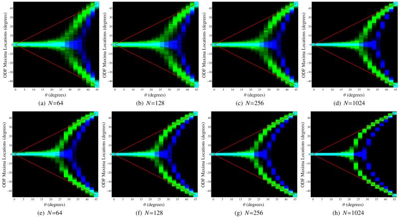
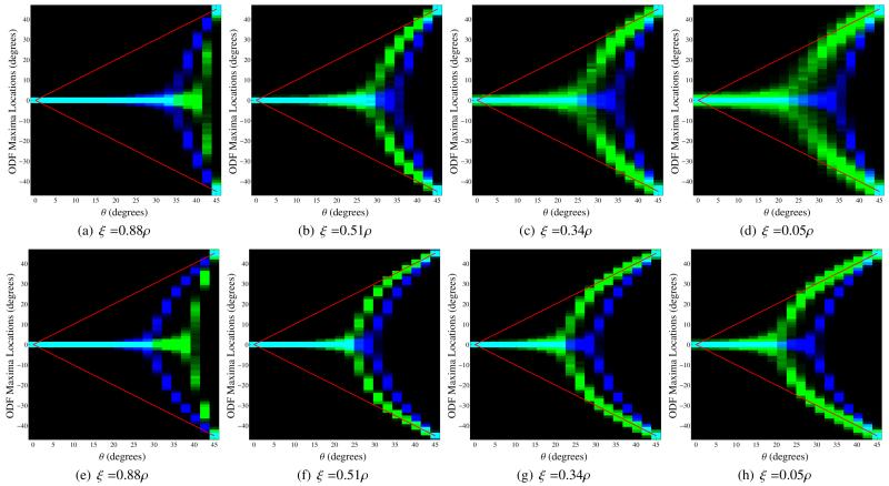
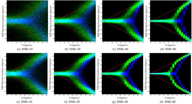
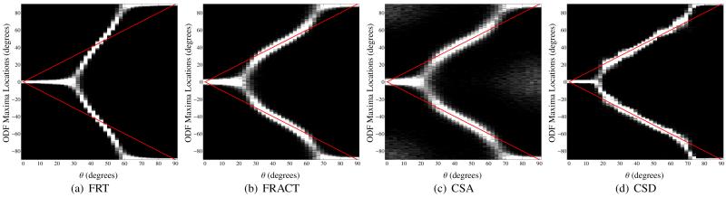
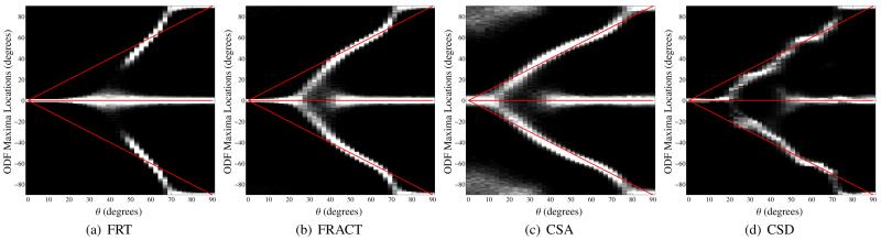
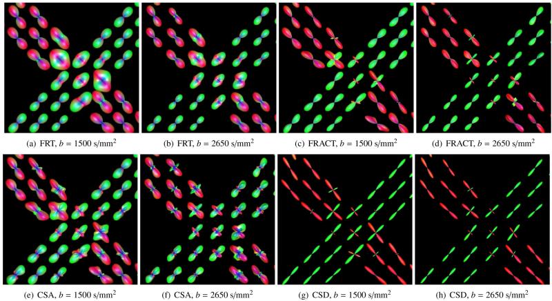
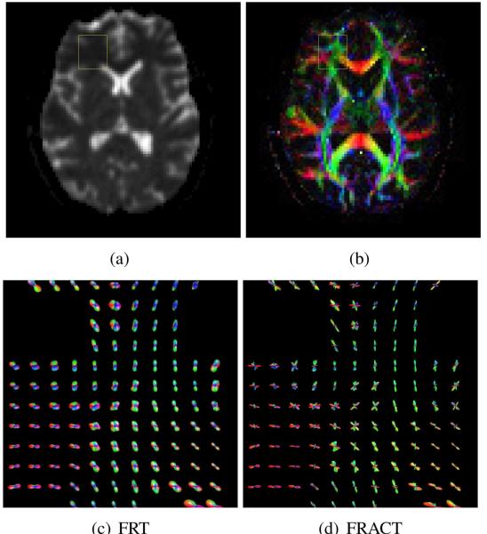
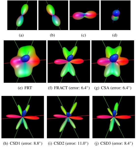
This paper presents a novel family of linear transforms that can be applied to data collected from the surface of a 2-sphere in three-dimensional Fourier space. This family of transforms generalizes the previously-proposed Funk-Radon Transform (FRT), which was originally developed for estimating the orientations of white matter fibers in the central nervous system from diffusion magnetic resonance imaging data. The new family of transforms is characterized theoretically, and efficient numerical implementations of the transforms are presented for the case when the measured data is represented in a basis of spherical harmonics. After these general discussions, attention is focused on a particular new transform from this family that we name the Funk-Radon and Cosine Transform (FRACT). Based on theoretical arguments, it is expected that FRACT-based analysis should yield significantly better orientation information (e.g., improved accuracy and higher angular resolution) than FRT-based analysis, while maintaining the strong characterizability and computational efficiency of the FRT. Simulations are used to confirm these theoretical characteristics, and the practical significance of the proposed approach is illustrated with real diffusion weighted MRI brain data. These experiments demonstrate that, in addition to having strong theoretical characteristics, the proposed approach can outperform existing state-of-the-art orientation estimation methods with respect to measures such as angular resolution and robustness to noise and modeling errors.


Figures

Figure 1
Figure 1
Illustration of the function pairs listed in Table 1. In each subfigure, the left image shows G(uTq) for q on the sphere, and the right image shows the magnitude of g~u(x,0,z) in the x-z plane, both for the case where u is oriented along the z-axis. Note that g~u(x,y,z) is axially symmetric about the z-axis. The function pairs are shown with (b) ξ = 0 and (c) ξ = 0.36ρ.
Figure 2
Figure 2
Illustration of FRACT for different choices of ξ. In each subfigure, the left image shows G(uTq) for q on the sphere, and the right image shows the magnitude of g~u(x,0,z) in the x-z plane, both for the case where u is oriented along the z-axis.
Figure 3
Figure 3
Magnitudes of the spherical harmonic eigenvalues for different transforms as a function of the spherical harmonic degree. Note that all of the eigenvalues in this plot are 0 for odd , and that these values are not shown. The eigenvalues for the FRACT transforms have been scaled by 2πξ2 for better comparison with the FRT, and ρ was assumed to be 1.
Figure 4
Figure 4
Sampling patterns with different numbers N of total measurements.
Figure 5
Figure 5
Images showing the magnitude of g~u(x,0,z) in the x-z plane for the FRT, in the presence of finite sampling of the sphere and truncation of the spherical harmonic series. (a)-(d) Results using L = 8. (e)-(h) Results using L = 32. Results can be compared to the ideal response function shown in Fig. 1(b).
Figure 6
Figure 6
Images showing the magnitude of g~u(x,0,z) in the x-z plane for the FRACT with parameter ξ = 0.51ρ, in the presence of finite sampling of the sphere and truncation of the spherical harmonic series. (a)-(d) Results using L = 8. (e)-(h) Results using L = 32. Results can be compared to the ideal response function shown in Fig. 2(b).
Figure 7
Figure 7
Qualitative comparison between the FRT and the FRACT at a b-value of 1000 s/mm2, in a two-tensor simulation with SNR=20, N =256 directions, ξ = 0.34ρ, and L = 8. Each image shows the mean ODF (solid) and the mean ODF plus two standard deviations (transparent). Results are shown for the (a)-(d) FRT and (e)-(h) FRACT, for crossing angles of (a,e) 47°, (b,f) 57°, (c,g) 76°, and (c,g) 90°.
Figure 8
Figure 8
Qualitative comparison between the FRT and the FRACT at a b-value of 2000 s/mm2, in a two-tensor simulation with SNR=20, N =256 directions, ξ = 0.34ρ, and L = 8. Each image shows the mean ODF (solid) and the mean ODF plus two standard deviations (transparent). Results are shown for (a)-(d) the FRT and (e)-(h) the FRACT, for crossing angles of (a,e) 47°, (b,f) 57°, (c,g) 76°, and (c,g) 90°.
Figure 9
Figure 9
Histograms for the locations of local maxima extracted from the FRT profiles (in blue) and the FRACT profiles (in green) for two simulated tensors in the x-y plane with orientation angles of −θ and +θ in polar coordinates. The color scale is set to saturate at 250 counts in a single histogram bin for improved visualization. The true orientations of the two tensors are also indicated using red lines. All simulations used SNR=80, ξ = 0.34ρ, and L = 8. The images from left to right show results for different numbers N of q-space samples. Results are shown for (a)-(d) a b-value of 1000 s/mm2 and (e)-(h) a b-value of 2000 s/mm2.
Figure 10
Figure 10
Histograms for the locations of local maxima extracted from the FRT profiles (in blue) and the FRACT profiles (in green) for two simulated tensors in the x-y plane with orientation angles of −θ and +θ in polar coordinates. The color scale is set to saturate at 250 counts in a single histogram bin for improved visualization. The true orientations of the two tensors are also indicated using red lines. All simulations used SNR=80, N = 256, and L = 8. The images from left to right show results for different values of the FRACT parameter ξ. Results are shown for (a)-(d) a b-value of 1000 s/mm2 and (e)-(h) a b-value of 2000 s/mm2.
Figure 11
Figure 11
Histograms for the locations of local maxima extracted from the FRT profiles (in blue) and the FRACT profiles (in green) for two simulated tensors in the x-y plane with orientation angles of −θ and +θ in polar coordinates. The color scale is set to saturate at 250 counts in a single histogram bin for improved visualization. The true orientations of the two tensors are also indicated using red lines. All simulations used ξ = 0.34ρ, N = 256, and L = 8. The images from left to right show results for different SNRs. Results are shown for (a)-(d) a b-value of 1000 s/mm2 and (e)-(h) a b-value of 2000 s/mm2.
Figure 12
Figure 12
Histograms for the locations of local maxima extracted from the (a) FRT profiles, (b) the FRACT profiles, (c) the CSA profiles, and (d) the CSD profiles for two simulated tensors in the x-y plane with orientation angles of −θ and +θ in polar coordinates. The gray scale is set to saturate at 40 counts in a single histogram bin for improved visualization. The true orientations of the two tensors are also indicated using red lines. All simulations used SNR=40, N = 256, and a b-value of 1500 s/mm2. Note that due to periodicity and symmetry relationships, the histogram for θ ∈ [45°, 90°) is a reversed and circularly-shifted version of the histogram for θ ∈ [0°, 45°).
Figure 13
Figure 13
Histograms for the locations of local maxima extracted from the (a) FRT profiles, (b) the FRACT profiles, (c) the CSA profiles, and (d) the CSD profiles for three simulated tensors in the x-y plane with orientation angles of −θ, 0, and +θ in polar coordinates. Note that, unlike the previous histograms, the separation angle for these histograms is θ rather than 2θ. The gray scale is set to saturate at 100 counts in a single histogram bin for improved visualization. The true orientations of the three tensors are also indicated using red lines. All simulations used SNR=80, N = 256, and a b-value of 5000 s/mm2.
Figure 14
Figure 14
ODFs reconstructed by applying (a)-(b) the FRT and (c)-(d) the FRACT to the FiberCup data. (a),(c) show results for the b = 1500 s/mm2 data, while (b),(d) show results for the b = 2650 s/mm2 data. The ODFs are color-coded by orientation.
Figure 15
Figure 15
Application of the FRT and the FRACT to in vivo human brain data. (a) A b = 0 s/mm2 image from a slice of interest. (b) The corresponding DTI fit, where image intensity corresponds to the fractional anisotropy of the tissue, while the image color corresponds to the orientation of the principal eigenvector of the estimated diffusion tensor. The yellow boxes in (a) and (b) indicate a region of interest (ROI) from the white matter core of the frontal lobe in which complicated fiber crossing patterns are known to occur. ODFs from the ROI are shown for (c) the FRT and (d) the FRACT.
Figure 16
Figure 16
Application of the FRT, the FRACT, CSA, and CSD to a mixture of fibers from in vivo human brain data. Data was combined from image voxels displaying a single dominant diffusion orientation, as shown in (a-d). FRT ODFs are shown for voxels corresponding to (a,b) forceps major, (c) genu of the corpus callosum, and (d) corticospinal tract. Reconstructions of the multi-fiber combined dataset are shown for (e) the FRT, (f) the FRACT, (g) CSA, (h) CSD1, (i) CSD2, and (j) CSD3. The lines shown in each image correspond to the dominant orientations estimated from (a-d). The figure captions show the maximum angular error between the estimated ODF maxima from the combined data and the ODF maxima from the original single-orientation data (this is not shown for the FRT, since the FRT fails to resolve all of the ODF peaks).

Similar articles

Cited by

References

    1. Aganj I, Lenglet C, Sapiro G, Yacoub E, Ugurbil K, Harel N. Reconstruction of the orientation distribution function in single- and multiple-shell q-ball imaging within constant solid angle. Magn. Reson. Med. 2010;64:554–566. - PMC - PubMed
    1. Alexander AL, Hasan KM, Lazar M, Tsuruda JS, Parker DL. Analysis of partial volume effects in diffusion-tensor MRI. Magn. Reson. Med. 2001;45:770–780. - PubMed
    1. Alexander DC. Multiple-fiber reconstruction algorithms for diffusion MRI. Ann. NY Acad. Sci. 2005;1064:113–133. - PubMed
    1. Alexander DC, Barker GJ, Arridge SR. Detection and modeling of non-Gaussian apparent diffusion coefficient profiles in human brain data. Magn. Reson. Med. 2002;48:331–340. - PubMed
    1. Anderson AW. Measurement of fiber orientation distributions using high angular resolution diffusion imaging. Magn. Reson. Med. 2005;54:1194–1206. - PubMed

Publication types