Observability of complex systems

Abstract

A quantitative description of a complex system is inherently limited by our ability to estimate the system's internal state from experimentally accessible outputs. Although the simultaneous measurement of all internal variables, like all metabolite concentrations in a cell, offers a complete description of a system's state, in practice experimental access is limited to only a subset of variables, or sensors. A system is called observable if we can reconstruct the system's complete internal state from its outputs. Here, we adopt a graphical approach derived from the dynamical laws that govern a system to determine the sensors that are necessary to reconstruct the full internal state of a complex system. We apply this approach to biochemical reaction systems, finding that the identified sensors are not only necessary but also sufficient for observability. The developed approach can also identify the optimal sensors for target or partial observability, helping us reconstruct selected state variables from appropriately chosen outputs, a prerequisite for optimal biomarker design. Given the fundamental role observability plays in complex systems, these results offer avenues to systematically explore the dynamics of a wide range of natural, technological and socioeconomic systems.

Fig. 1.

Graphical approach. (A) Chemical reaction system with 11 species (A,B,…,J,K) involved in four reactions. Because two reactions are reversible, we have six elementary reactions. (B) Balance equations of the chemical reaction system shown in A. Concentrations of the 11 species are denoted by x₁, x₂,…,x₁₀, x₁₁, respectively. Rate constants of the six elementary reactions are given by k₁, k₂,…,k₆, respectively. Balance equations are derived using the mass-action kinetics. (C) Inference diagram is constructed by drawing a directed link (x_i → x_j) if x_j appears in the right-hand side of x_i’s balance equation shown in B. SCCs, which are the largest subgraphs chosen such that there is a directed path from each node to every other node in the subgraph, are marked with dashed circle; root SCCs, which have no incoming links, are shaded in gray. A potential minimum set of sensor nodes, whose measurements allow us to reconstruct the state of all other variables (metabolite concentrations), is shown in red.

Fig. 2.

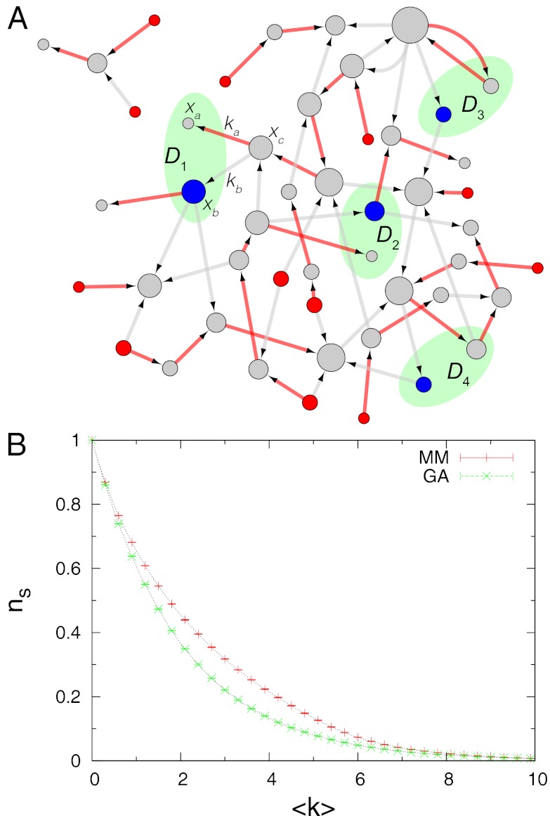
Sensor nodes in linear systems. For linear systems and , the minimum set of sensors sufficient for full observability can be calculated exactly using the maximum matching (MM) algorithm (17), whereas the necessary sensor set is provided by the GA. (A) Erdös–Rényi (ER) network with mean degree 〈k〉 ∼ 3.5. The necessary sensor set predicted by GA is shown in red; the additional nodes that we also need to be monitor to obtain full observability are shown in blue. Hence, red and blue nodes together form the sufficient sensor set. Dilations are highlighted in green. Dilation occurs if there is a subset S of the nodes (i.e., the state variables) such that , where the neighborhood set of a set S is defined to be the set of all nodes j where a directed edge exists from j to a node in S (6). Such dilations can be identified via MM algorithm. If the blue nodes are not monitored then their dilations will cause symmetries that leave the outputs and derivatives of outputs invariant. For example, in A, if x_b is not monitored, the subset S₁ = {x_a, x_b} will cause a dilation D₁ and a family of symmetries that leave the outputs (and their derivatives) invariant because . (B) n_s representing the fraction of sensors, predicted by GA (green “x”) or MM (red “+”), as a function of 〈k〉 for ER random networks of size n = 10⁴. The results are averaged over 10 realizations with error bars defined as SEM. The difference between the two curves indicates that for such linear systems GA underestimates the necessary sensor set. (Similar results are also obtained for linear systems with scale-free random network topology; refs. , .) We find, however, that for nonlinear dynamics, the GA-identified nodes can be both sufficient and necessary for observability, as symmetries in state variables are very unlikely for large systems.

Fig. 3.

Biochemical reaction systems and their inference diagrams. (A) Simplified glycolytic reaction map (20), where the symbols denote G6P, F6P, TP, F2-6BP, ATP (adenosine 5′-triphosphate), and ADP (adenosine 5′-diphosphate). Source (glucose) and sinks (G1P and Pyr) are also included in this model. Different chemical species are shown in different colors. (B) Inference diagram of the reaction system shown in A consists of a nonroot SCC of nine species (marked with dashed circle) and a root SCC of one species––the pure product Pyr (shaded in gray), hence indicating that the system can be observed through monitoring the concentration of Pyr only. (C) Simple model of ligand binding (23). The symbols denote Epo, EpoR, Epo_EpoR, Epo_EpoR_i, dEpo_i, and dEpo_e, marked with different colors. B_max is the maximal amount of receptor at the cell membrane. (D) Inference diagram of the reaction system shown in C consists of a nonroot SCC of four species (marked with dashed circles) and two root SCCs (shaded in gray). Each root SCC contains one pure product. The system can be observed through monitoring the concentrations of the two pure products, dEpo_i and dEpo_e.

References

-
- Diop S, Fliess M. 1991. On nonlinear observability, Proceedings of ECC’91 (Hermès, Paris), Vol 1, pp 152–157.
- Diop S, Fliess M. 1991. Nonlinear observability, identifiability, and persistent trajectories, Proceedings of the 30th IEEE Conference on Decision and Control (IEEE Press, New York), Vol 1, pp 714–719.
- Kalman RE. Mathematical description of linear dynamical systems. J Soc Ind Appl Math Ser A. 1963;1(2):152–192.
- Luenberger DG. Introduction to Dynamic Systems: Theory, Models, & Applications. New York: Wiley; 1979.
- Sedoglavic A. A probabilistic algorithm to test local algebraic observability in polynomial time. J Symb Comput. 2002;33(5):735–755.
Publication types
MeSH terms
LinkOut - more resources
Full Text Sources
Other Literature Sources