Adaptation improves neural coding efficiency despite increasing correlations in variability

Abstract

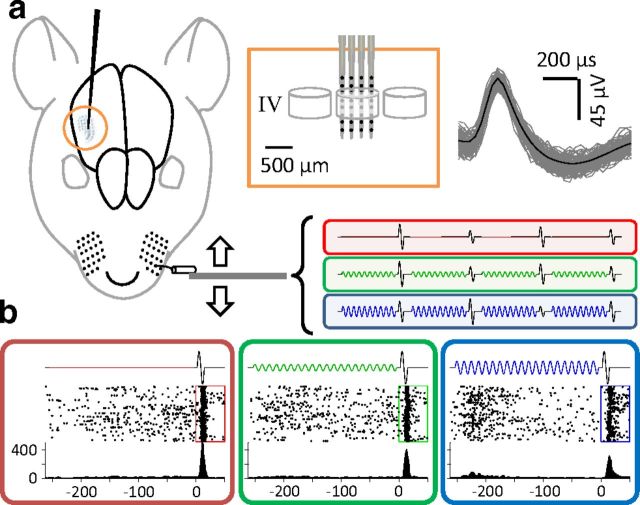
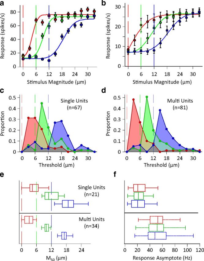
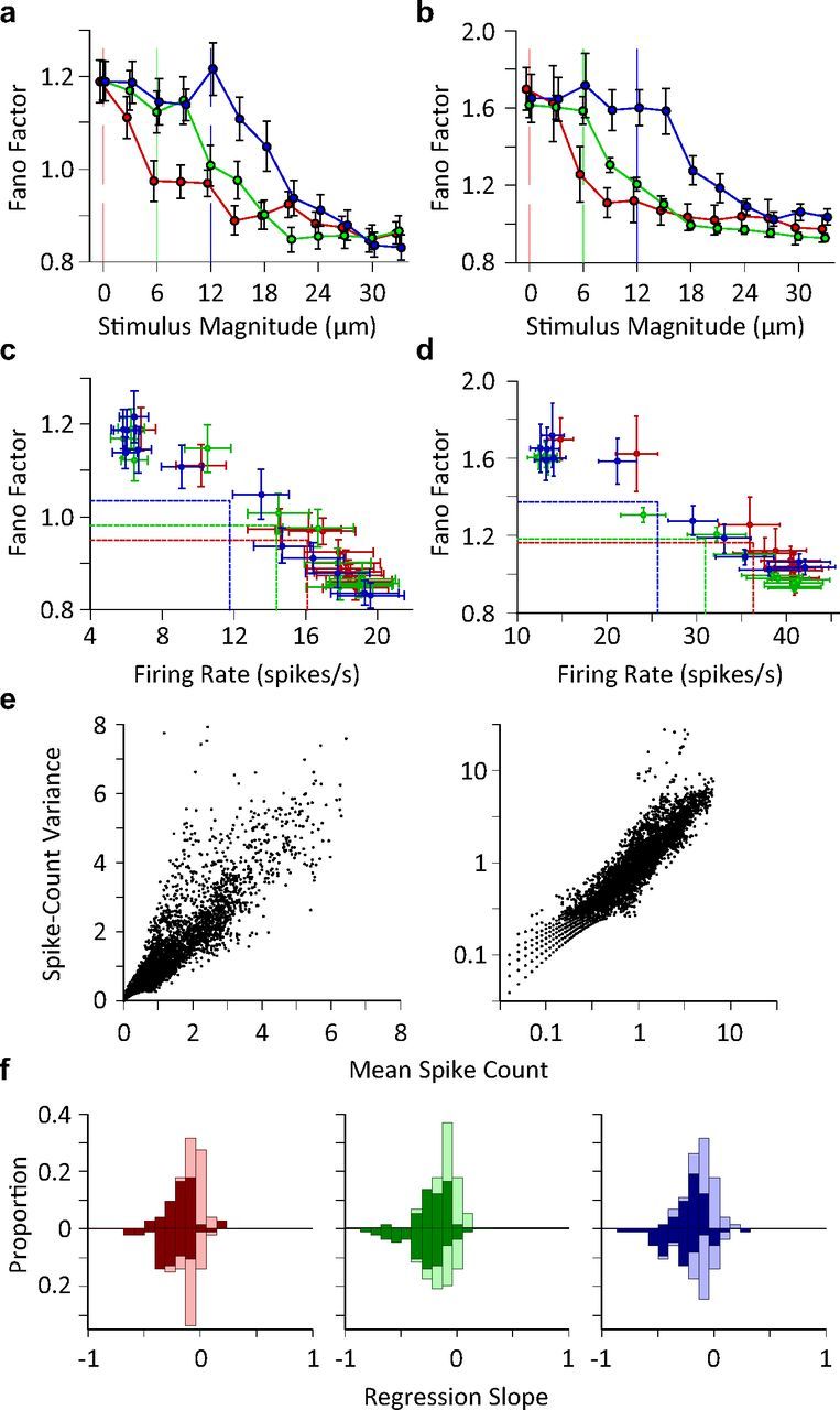
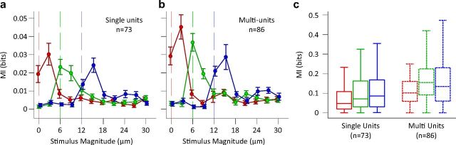
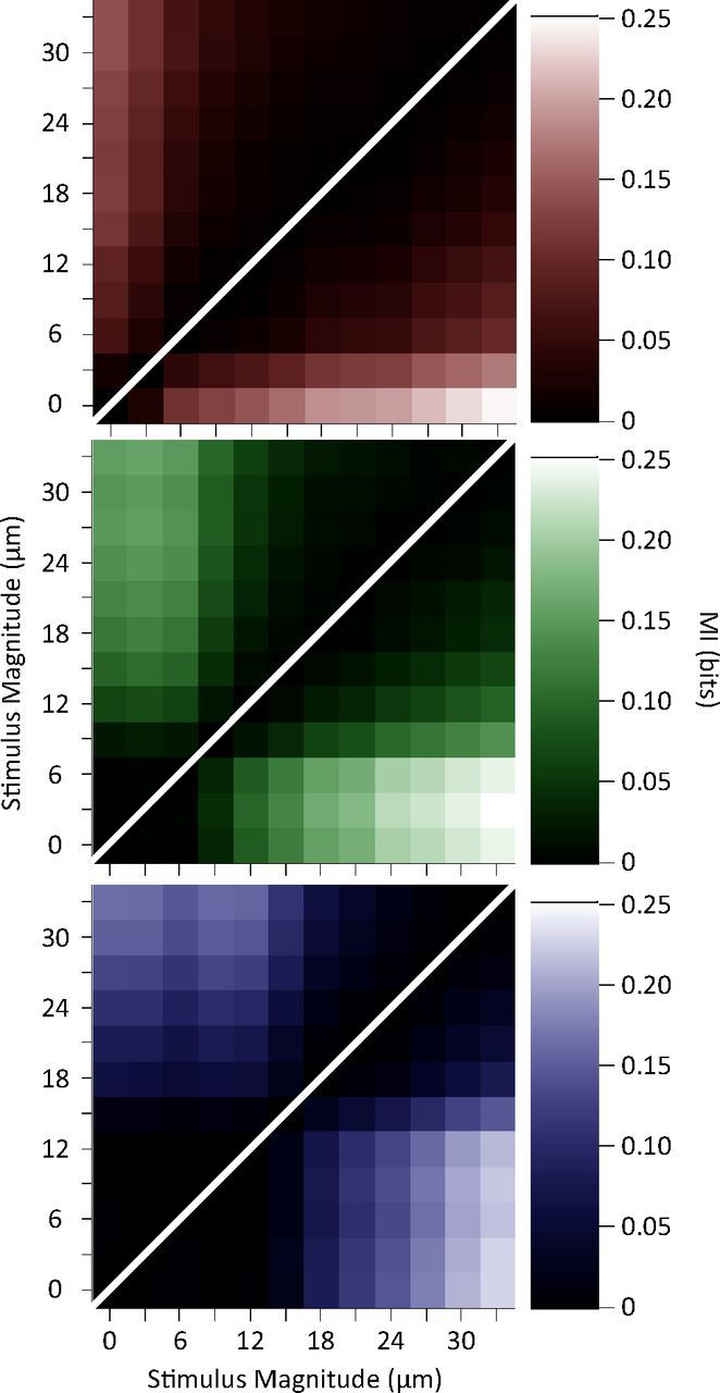
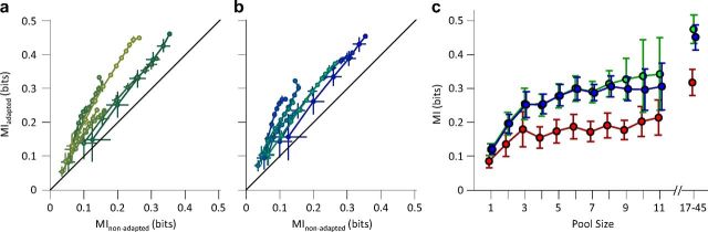
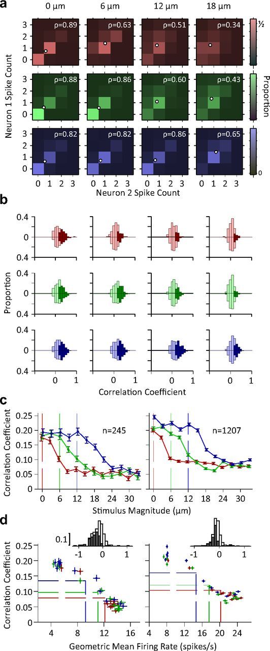
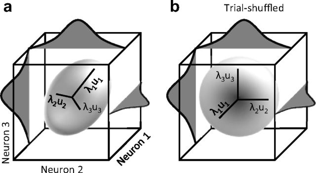
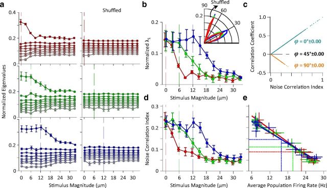
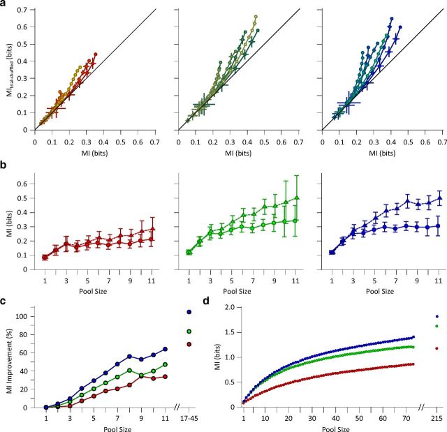
Exposure of cortical cells to sustained sensory stimuli results in changes in the neuronal response function. This phenomenon, known as adaptation, is a common feature across sensory modalities. Here, we quantified the functional effect of adaptation on the ensemble activity of cortical neurons in the rat whisker-barrel system. A multishank array of electrodes was used to allow simultaneous sampling of neuronal activity. We characterized the response of neurons to sinusoidal whisker vibrations of varying amplitude in three states of adaptation. The adaptors produced a systematic rightward shift in the neuronal response function. Consistently, mutual information revealed that peak discrimination performance was not aligned to the adaptor but to test amplitudes 3-9 μm higher. Stimulus presentation reduced single neuron trial-to-trial response variability (captured by Fano factor) and correlations in the population response variability (noise correlation). We found that these two types of variability were inversely proportional to the average firing rate regardless of the adaptation state. Adaptation transferred the neuronal operating regime to lower rates with higher Fano factor and noise correlations. Noise correlations were positive and in the direction of signal, and thus detrimental to coding efficiency. Interestingly, across all population sizes, the net effect of adaptation was to increase the total information despite increasing the noise correlation between neurons.

Figure 1.

Multi-electrode array recording in rat barrel cortex. a, An illustration of the whisker barrels in rat S1 cortex. Inset shows a close-up schematic of the recording probe's penetration of a barrel and the isolated spikes of a typical single unit recorded from Barrel D4. b, Each panel shows response of the sample neuron to the 30 μm test stimulus in each adaptation condition: red, no adaptation; green, 6 μm magnitude adaptation; blue, 12 μm magnitude adaptation. Middle trace is a raster plot of spiking activity over 100 trials. The bottom graph is the peristimulus time histogram. Spike rate is calculated in a 5ms long bin that slides in 1 ms steps.

Figure 2.

Single unit and population response characteristics in different adaptation states. a, Amplitude response functions of the example neuron from Figure 1. Data points in red indicate response to the test stimulus following no adaptation; points in green and blue indicate response following adaptation to 6 and 12 μm vibration (this convention will be used henceforth). Vertical lines represent the magnitude of the adapting stimulus. Continuous lines represent the best fit of a cumulative Gaussian function to each of the three neuronal response functions. Error bars represent standard error of means across trials. b, Average population response functions. The responses of simultaneously recorded units were averaged to produce a population spike count for individual sessions with a minimum of 5 units. The population spike counts were then averaged across sessions (n = 8). Conventions and fitting are as described in a. Error bars represent the standard error of means across sessions. c, The histogram of the distribution of neuronal thresholds for single units. d, As in c but for clusters of multiunits. e, Distribution of the M₅₀ for single-units (top) and multiunit clusters (bottom). Whiskers of the box plot indicate the extent of the M₅₀ distribution, ends of the boxes represent the upper and lower quartiles, and the bisection line of the boxes indicates the median of the distribution. Vertical lines indicate the magnitude of adapting stimulus. f, Distribution of maximum response rate of fitted cumulative Gaussians for the units in e.

Figure 3.

Trial-to-trial variations in neuronal response. a, Single unit Fano factor as a function of stimulus intensity. The plot includes 64 single units as 9 (out of 73) units had zero firing rate in one or more conditions and, consequently, calculating the Fano factor meant division by zero. Each data point represents one stimulus. Error bars indicate standard error of means across neurons. b, as in a but for multiunit clusters (n = 69). c, Fano factor as a function of average firing rate for single neurons. Each data point represents the average Fano factor versus the average firing rate across recordings for a unique stimulus. The horizontal and vertical lines show the mean of average values (center of the distribution of data points) along y- and x-axes for each adaptation state. d, As in c, but for multiunit clusters from b. e, Spike count variance as a function of average spike count. Spike count is calculated over a 50 ms window post stimulus onset. Each data point corresponds to a unique neuron-stimulus-adaptation state triplet. Right panel contains the same data as in the left panel; however, the axes are in logarithmic scale for a clear demonstration of low firing rate regimes. f, The histogram of the linear regression slope of the Fano factor with respect to the z-scored neuronal activity for single units (upward bars) and multiunit clusters (downward bars) separately plotted for every adaptation state. The dark bars correspond to recordings with a significant linear regression (p < 0.05).

Figure 4.

Information transmission in single- and multi-units. a, Mutual information between responses of single neurons and pairs of stimuli (with a magnitude difference of Δs = 3 μm). Abscissa is the smaller stimulus magnitude of each stimulus pair. Vertical lines indicate the amplitude of the adaptors. Error bars are standard error of means across single neurons. b, As in a, but for multiunit clusters. c, Mutual information between neural responses and the total set of stimuli (n = 12). Box and whisker plots and colors follow previous conventions.

Figure 5.

Discriminability between pairs of stimuli measured as the mutual information between responses of neurons and each stimulus pair. The brightness of each element in the graph gives the mutual information value about that stimulus pair averaged across single units (top left triangle) and multiunit clusters (bottom right triangle).

Figure 6.

Population coding efficiency. a, The mutual information in the 6 μm adaptation state (ordinate) and nonadapted state (abscissa). Various population sizes within a session are connected with a line. Multiple levels of brightness are used for better visibility. For each population size, the information content of all possible selections of that size were averaged within session. Error bars indicate the standard error of means. b, As in a, but for 12 μm adaptation state (ordinate) compared to the nonadapted state (abscissa). The y-axis is the same as the one in a. c, Mutual information between pooled single-unit responses and the total set of stimuli as a function of pool size. Different adaptation conditions are colored as per convention. Error bars are standard error of means across recording sessions. The data points after the break in the abscissa include multiunit clusters with the single-unit data to provide the full population response in each session. We estimate that these recordings consisted of between 17 and 45 single units.

Figure 7.

Correlations in variability across pairs of neurons. a, Color indicates the proportion of joint spike counts for a pair of simultaneously recorded single neurons. White circles indicate mean spike counts for each stimulus. The Pearson's correlation coefficient of the spike counts is indicated by ρ for each panel. b, Histogram of pairwise correlation coefficients across all possible simultaneously recorded single unit pairs (n = 245; upward bars) and other neuronal pairs (n = 1207; downward bars). Dark colors indicate correlation coefficients that are significantly different from zero (p < 0.05). c, The mean Pearson's correlation coefficient across all possible pairs of single units (left) and other neuronal recording pairs (right) as a function of stimulus intensity. Error bars indicate standard error of means. d, Pearson's correlation coefficient as a function of geometric mean firing rate of neuronal pairs. Each data point represents average correlation coefficient against geometric mean firing rate averaged across all pairs of simultaneously recorded single neurons (left; n = 245) or averaged across all other possible pairs of recordings excluding pairs of single neurons (right; n = 1207). Every data point represents one stimulus. Dashed lines show the mean of average values (center of the distribution of data points) for each adaptation state. The insets depict the histogram of regression slopes of Pearson's correlation against average firing rate for individual pairs (single unit pairs on the left, other pairs on the right). For each pair, regression analysis was performed across all stimuli and adaptation states. Dark bars indicate the cases that linear regression was significant (p < 0.05).

Figure 8.

Schematic illustration of neuronal response covariation for a population of 3 neurons. a, Each dimension represents the z-scored activity of one neuron. The marginal distribution of responses for individual neurons are plotted on their corresponding axes. PCA is used to characterize the shape of the population response distributions in terms of the maximum amount of stretch (highest eigenvalue, λ₁) and its direction (first eigenvector, u₁). b, Shuffling trial sequence across neurons eliminates the covariation without affecting the marginal distributions.

Figure 9.

Correlations in variability in the neuronal population activity as revealed by principal component analysis. a. Left panels: z-scored neuronal responses were used to calculate normalized eigenvalues which are plotted as a function of test stimulus amplitude for each adaptation condition, for populations of 8 simultaneously recorded single units. Right panels: the average normalized eigenvalues with the order of trials shuffled. Error bars are the standard error of the means across recording sessions which contain at least 8 single neurons (n = 5). Vertical lines indicate the magnitude of the adaptor. b, Replotting the first eigenvalues (λ₁) from a for direct comparison across adaptation states. The shuffled values are subtracted to remove the bias and provide a direct measure of noise correlation. Error bars are the standard error of means across sessions. The inset demonstrates the distribution of angles between the first eigenvector (u₁) and the diagonal line. This eigenvector is referred to as noise direction. For clarity of illustration, the histogram of the shuffled angles is scaled down by a factor of 3. As the noise direction did not change as a function of stimulus amplitude, the histogram is plotted for all stimuli. c, The relationship between noise correlation index (abscissa) and Pearson's correlation coefficient (ordinate) for neuronal pairs. Each data point corresponds to a unique neuron pair recorded in a unique stimulus-adaptation condition. ϕ denotes the angle between the noise direction and the diagonal line. d, The noise correlation index as a function of stimulus amplitude averaged across sessions containing at least five simultaneously recorded units (n = 8). Error bars are standard error of mean across sessions. e, The noise correlation indices from d but replotted as a function of average population firing rate. Each data point corresponds to the average noise correlation index for each stimulus and adaptation condition. The average population firing rate was calculated by averaging firing rates across neurons and trials within each session. The solid tick lines indicate the linear regressions for each adaptation state. The horizontal and vertical lines show the mean of average values (center of the distribution of data points) for each adaptation state.

Figure 10.

Noise correlation reduces the information efficiency. a, Mutual information for simultaneously recorded single neurons (abscissa) compared with the mutual information for the shuffled responses (ordinate) for each session. The shuffling procedure was repeated 50 times, and the average mutual information value was plotted as MI_{trial-shuffled}. Each line connects different population sizes within a session. Multiple levels of brightness are used for better visibility. For each population size, the information content of all possible selections of that size was averaged within session. Error bars indicate the standard error of means. b, Solid lines with circles as marker indicate mutual information for the simultaneously recorded neural responses (carried over from Fig. 6). Dashed lines with triangles as marker indicate mutual information for the same neuronal responses, but now with a shuffled trial structure. Error bars are the standard error of means across eight recording sessions. c, The percentage improvement in mutual information after shuffling as a function of pool size. d, Mutual information between stimuli and pooled neuronal response across all sessions. Trials of the simultaneously recorded neurons were shuffled to remove noise correlation. For each population size, the information content of 1000 random selections of that size was averaged. This was done with the exception of the population sizes of 1, 72, and 73 neurons, where the number of possible selections was limited to 73, 73, and 1, respectively. The data points after the break in the abscissa includes multiunit clusters with the single-unit data to provide the full population response across all sessions (n = 16). From the firing rates, we estimate that the total population consisted of ∼215 single units.

References

1. Abbott LF, Dayan P. The effect of correlated variability on the accuracy of a population code. Neural Comput. 1999;11:91–101. - PubMed
1. Abbott LF, Rajan K, Sompolinsky H. Interactions between intrinsic and stimulus-evoked activity in recurrent neural networks. In: Ding M, Glanzman DL, editors. The Dynamic brain: an exploration of neuronal variability and its functional significance. New York: Oxford UP; 2011. pp. 65–82.
1. Adibi M, Arabzadeh E. A comparison of neuronal and behavioral detection and discrimination performances in rat whisker system. J Neurophysiol. 2011;105:356–365. - PubMed
1. Adibi M, Diamond ME, Arabzadeh E. Behavioral study of whisker-mediated vibration sensation in rats. Proc Natl Acad Sci U S A. 2012;109:971–976. - PMC - PubMed
1. Ahissar E, Knutsen PM. Object localization with whiskers. Biological Cybernetics. 2008;98:449–458. - PubMed
Publication types
LinkOut - more resources