. 2013 Feb 8:6:359.
doi: 10.3389/fnhum.2012.00359. eCollection 2012.

A model-based approach to trial-by-trial p300 amplitude fluctuations

Affiliations

A model-based approach to trial-by-trial p300 amplitude fluctuations

Antonio Kolossa et al. Front Hum Neurosci. .

Abstract

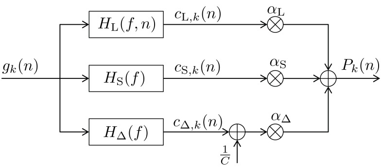
It has long been recognized that the amplitude of the P300 component of event-related brain potentials is sensitive to the degree to which eliciting stimuli are surprising to the observers (Donchin, 1981). While Squires et al. (1976) showed and modeled dependencies of P300 amplitudes from observed stimuli on various time scales, Mars et al. (2008) proposed a computational model keeping track of stimulus probabilities on a long-term time scale. We suggest here a computational model which integrates prior information with short-term, long-term, and alternation-based experiential influences on P300 amplitude fluctuations. To evaluate the new model, we measured trial-by-trial P300 amplitude fluctuations in a simple two-choice response time task, and tested the computational models of trial-by-trial P300 amplitudes using Bayesian model evaluation. The results reveal that the new digital filtering (DIF) model provides a superior account of the trial-by-trial P300 amplitudes when compared to both Squires et al.'s (1976) model, and Mars et al.'s (2008) model. We show that the P300-generating system can be described as two parallel first-order infinite impulse response (IIR) low-pass filters and an additional fourth-order finite impulse response (FIR) high-pass filter. Implications of the acquired data are discussed with regard to the neurobiological distinction between short-term, long-term, and working memory as well as from the point of view of predictive coding models and Bayesian learning theories of cortical function.

Keywords: Bayesian surprise; P300; digital filtering; event-related brain potentials; predictive surprise; single trial EEG.


Figures

Figure 1
Figure 1
Block diagram of the new digital filter (DIF) model with input gk(n) in (10) and output Pk(n) in (9), digital filter transfer functions H(f) with 0 ≤ f ≤ fs/2, a stimulus presentation rate of fs (= 2/3 Hz), and probability normalizing constant 1/C.
Figure 2
Figure 2
Block diagram of a first-order infinite impulse response length (IIR) filter with transfer function HS(f ) equivalent to (11) or (12). Elements formula image 
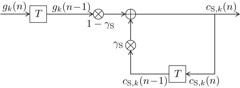
denote a delay of one trial. At the adder element ⊕, updating of the weighted output γS·cS,k(n − 1) of the last trial n − 1 with the weighted input (1 − γSgk(n − 1) of the last trial results in the current output cS,k(n). Note that via γS·cS,k(n − 1), all preceding inputs (and outputs) influence the current output, though for the short-term memory, the influence of trials not in the recent past is negligible.
Figure 3
Figure 3
Block diagram of a first-order infinite impulse response length (IIR) filter with transfer function HL(f,n) equivalent to (13) or (14). Elements formula image 
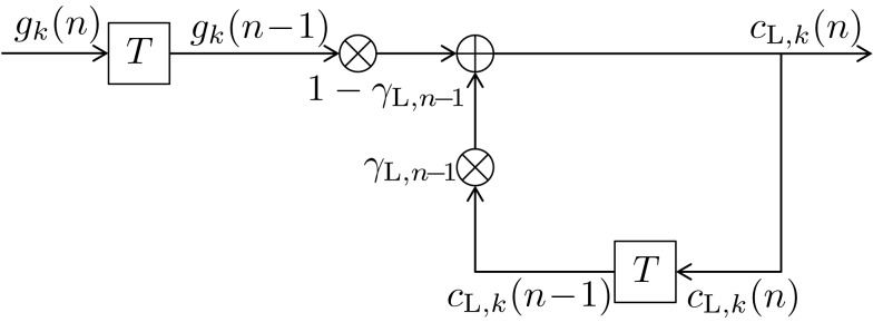
denote a delay of one trial. At the adder element ⊕, updating of the weighted output γL,n−1·cL,k(n − 1) of the last trial n − 1 with the weighted input (1 − γL,n−1gk(n − 1) of the last trial results in the current output cL,k(n). Note that via γL,n−1·cL,k(n − 1), all preceding inputs (and outputs) influence the current output.
Figure 4
Figure 4
Amplitude responses of the long-term (HL(f,n), dash-dotted and solid low-pass curves), short-term (HS(f ), dashed low-pass curve) and alternation (HΔ(f ), dashed high-pass curve) filters of the DIF model as a function of the input signal frequency f (logarithmic scale!). The dynamic long-term filter (dash-dotted and solid curves) is shown for n = 1 and n = N = 192.
Figure 5
Figure 5
Grand-average waveforms (A,B) and topographic maps (C,D) of P300 amplitudes. (A,C) Probability effect on P300 amplitudes in the [0.3, 0.7] probability category. (C) The probability maps show the scalp topography of the rare-frequent difference wave in the [0.3, 0.7] probability category at various points in time (276–396 ms, divided into five windows of 24 ms each). (B,D) Sequence effect on P300 amplitudes in the [0.5, 0.5] probability category. Note that sequences of four successive stimuli are illustrated; a signifies a particular stimulus (b the other one). Note further that the two solid traces, originating from the abaa and the baba sequences, respectively, show reversed P300 amplitudes. Specifically, for the single -b- sequence abaa, the P300 waveform lies amongst those from dual -bb- sequences, whereas for the dual -bb- sequence baba, the P300 waveform appears indistinguishable from the waveforms from single -b- sequences. As further detailed in the Discussion, this amplitude reversal is attributed to the disconfirmation of alternation expectation in the abaa sequence, was well as to the confirmation of alternation expectation in the baba sequence. (D) Sequence maps show the scalp topography of the bbba-aaaa difference wave in the [0.5, 0.5] probability category at various points in time (292–412 ms, divided into five time windows of 24 ms each).
Figure 6
Figure 6
Log-Bayes factors, ln(BFDIF − XXX), under variation of the model parameters. The upper contour always shows ln(BFDIF − MAR), the lower one ln(BFDIF − SQU). The “V” marks the parameter combination with the maximum log-Bayes factor, cf. Table 3. (A) Variation of the free short-term parameters βS and αS. (B) Variation of the free long-term parameters τ1 and τ2. In order to keep the lower contour visible, the log-Bayes factors for the 10 smallest values for τ2 are not displayed. (C) Variation of the free alternation parameters γΔ,2 and αΔ.
Figure 7
Figure 7
Timeline plots for one exemplary participant. (A,C,E) Probability category [0.5, 0.5]. (B,D,F) Probability category [0.3, 0.7]. Green symbols denote the stimuli s(n) ∈ {1,2} as they occurred. (A,B) Subjective probabilities Pk=1(n) and expectancies Ek=1(n) from (5), (7), and (9) for MAR, SQU, and DIF, respectively, for stimulus s(n) = 1. (C,D) Subjective probabilities Pk=s(n)(n) and expectancies Ek=s(n)(n) for the actually presented stimulus k = s(n). (E,F) The measured P300 estimates Y(n) and the model-based P300 estimates Y^(n) of the MAR, SQU, and DIF models, respectively.
Figure 8
Figure 8
Tree diagrams of measured P300 estimates Y(n) and model-based P300 estimates Y^(n) as a function of the sequence of preceding stimuli. Within each order (0–3), the stimulus sequence is labeled, and related sequences are connected by lines. (A) For both stimuli on probability category [0.5, 0.5]. (B) For the frequently occurring stimulus b on probability category [0.3, 0.7]. (C) For the rarely occurring stimulus a on probability category [0.3, 0.7].
Figure 9
Figure 9
Block diagram of the fourth-order finite impulse response (FIR) filter HΔ(f ). Elements formula image 
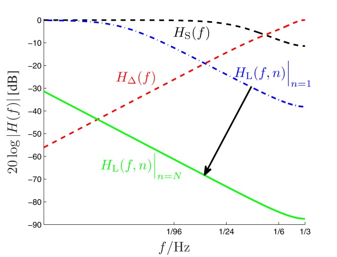
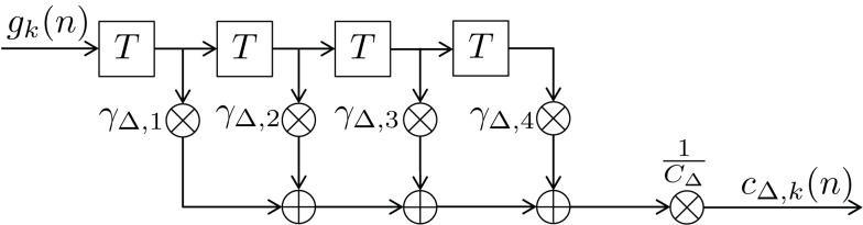
represent a delay of one trial, the multipliers γΔ,i compose the filter coefficients and CΔ constitutes a normalizing constant.
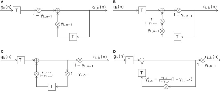
Figure A1
Figure A1
Illustration of the equivalence of the digital filter (14) (Figure 3) to the count function as in (13). (A) Block diagram of the DIF model’s long-term memory filter of Figure 3 and (14) with input signal gk(n) and output signal cL,k(n). (B) Block diagram of a filter equivalent to (A), where the multiplier (1 − γL,n − 1) has been moved to the right. (C) Block diagram of a filter equivalent to (B), where the multiplier (1 − γL,n − 1) has been moved even further to the right. (D) Block diagram of a filter equivalent to (C), where the multiplier γL,n − 1/(1 − γL,n − 1) has been moved to the right of the delay unit in the lower branch.
Figure A2
Figure A2
The dynamics of the coefficients γL,n (solid) and βL,n (dashed) over trials n = 1, …, N, with N = 192.

Similar articles

Cited by

References

    1. Alba J. W., Chromiak W., Hasher L., Attig M. S. (1980). Automatic encoding of category size information. J. Exp. Psychol. Hum. Learn. 6, 370–37810.1037/0278-7393.6.4.370 - DOI
    1. Baddeley A. (2003). Working memory: looking back and looking forward. Nat. Rev. Neurosci. 4, 829–83910.1038/nrm1251 - DOI - PubMed
    1. Baldi P., Itti L. (2010). Of bits and wows: a Bayesian theory of surprise with applications to attention. Neural Netw. 23, 649–66610.1016/j.neunet.2009.12.007 - DOI - PMC - PubMed
    1. Barceló F., Periáñez J. A., Nyhus E. (2008). An information theoretical approach to task-switching: evidence from cognitive brain potentials in humans. Front. Hum. Neurosci. 1:13.10.3389/neuro.09/013.2007 - DOI - PMC - PubMed
    1. Barlow H. (2001). Redundancy reduction revisited. Network 12, 241–25310.1088/0954-898X/12/3/301 - DOI - PubMed

LinkOut - more resources