Neural control and adaptive neural forward models for insect-like, energy-efficient, and adaptable locomotion of walking machines

Abstract

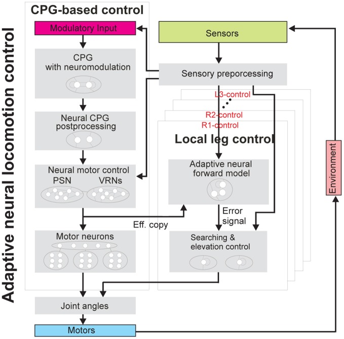
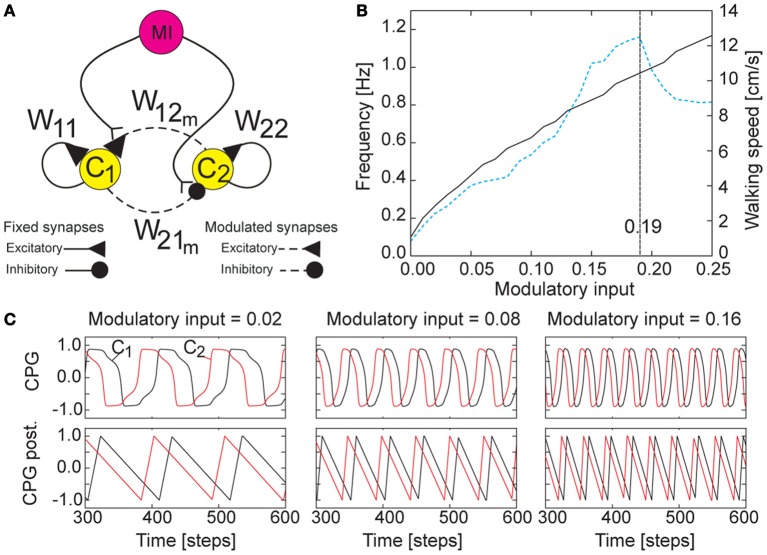
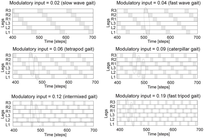
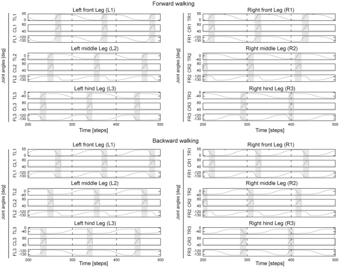
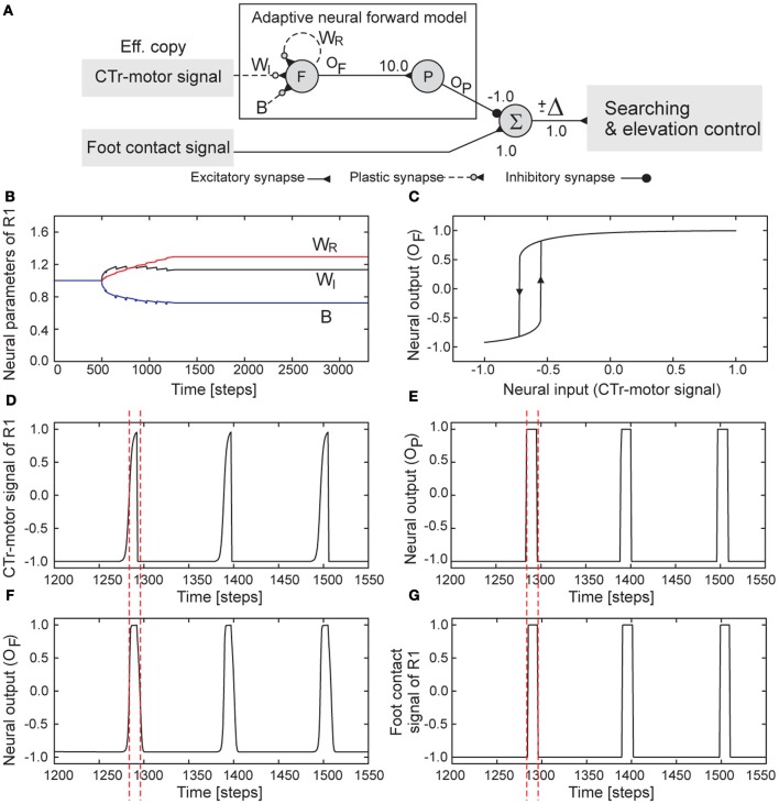
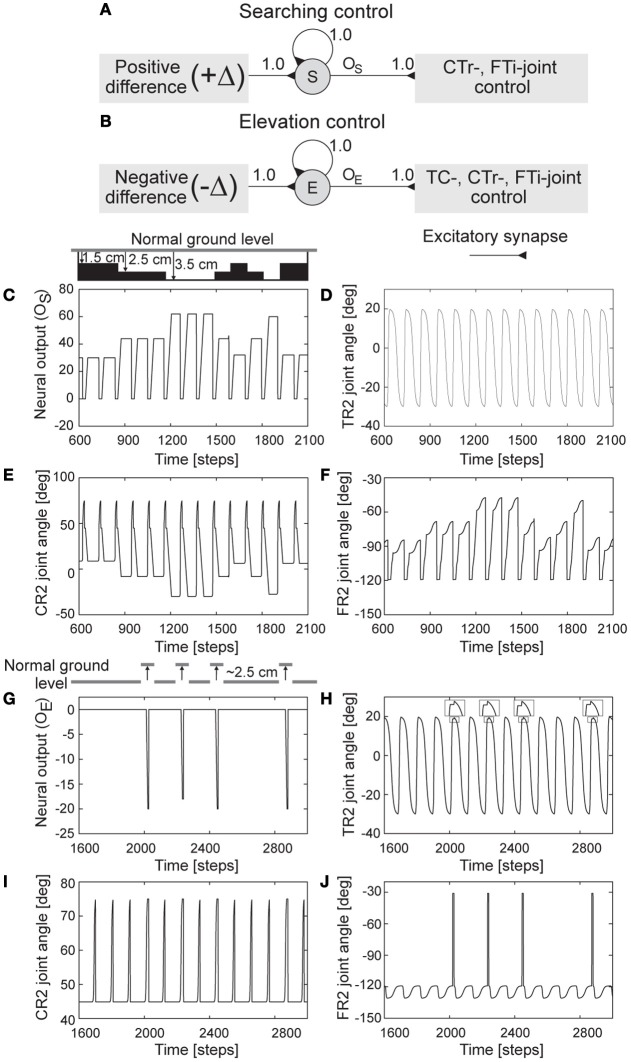
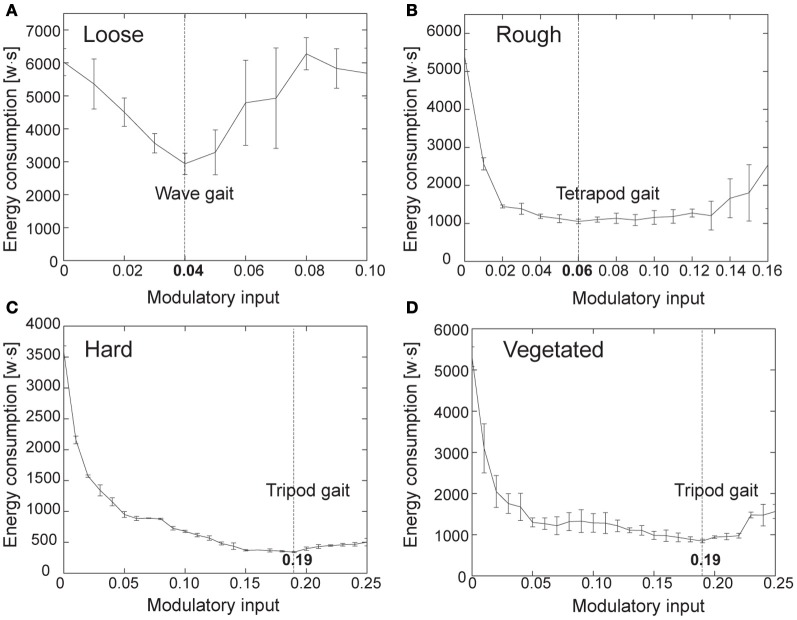
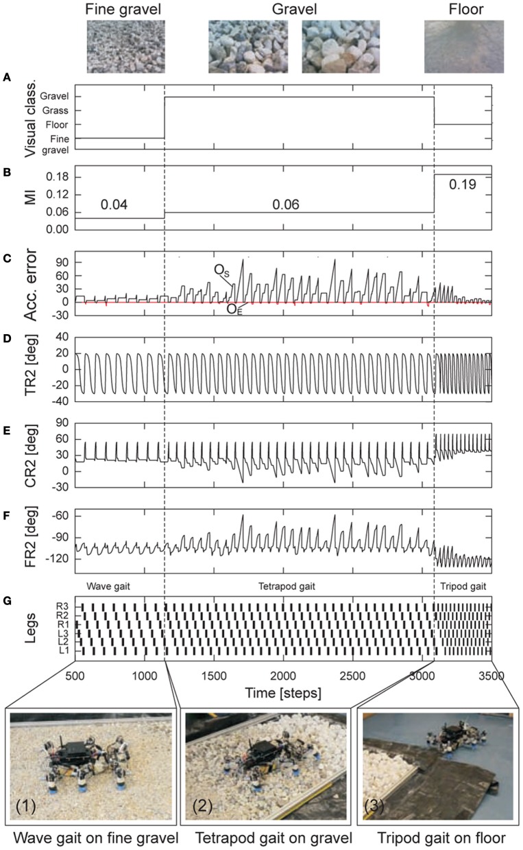
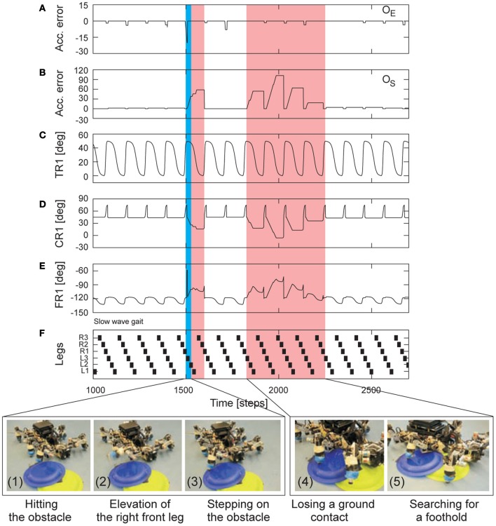
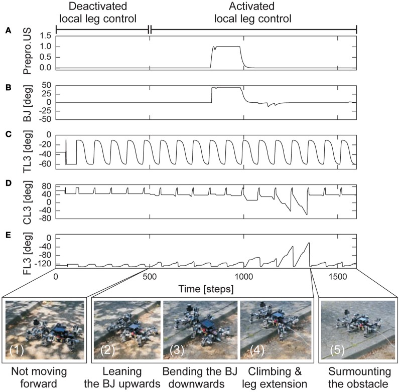
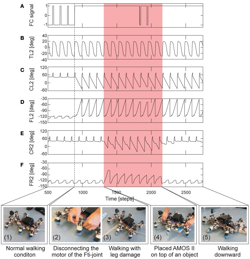
Living creatures, like walking animals, have found fascinating solutions for the problem of locomotion control. Their movements show the impression of elegance including versatile, energy-efficient, and adaptable locomotion. During the last few decades, roboticists have tried to imitate such natural properties with artificial legged locomotion systems by using different approaches including machine learning algorithms, classical engineering control techniques, and biologically-inspired control mechanisms. However, their levels of performance are still far from the natural ones. By contrast, animal locomotion mechanisms seem to largely depend not only on central mechanisms (central pattern generators, CPGs) and sensory feedback (afferent-based control) but also on internal forward models (efference copies). They are used to a different degree in different animals. Generally, CPGs organize basic rhythmic motions which are shaped by sensory feedback while internal models are used for sensory prediction and state estimations. According to this concept, we present here adaptive neural locomotion control consisting of a CPG mechanism with neuromodulation and local leg control mechanisms based on sensory feedback and adaptive neural forward models with efference copies. This neural closed-loop controller enables a walking machine to perform a multitude of different walking patterns including insect-like leg movements and gaits as well as energy-efficient locomotion. In addition, the forward models allow the machine to autonomously adapt its locomotion to deal with a change of terrain, losing of ground contact during stance phase, stepping on or hitting an obstacle during swing phase, leg damage, and even to promote cockroach-like climbing behavior. Thus, the results presented here show that the employed embodied neural closed-loop system can be a powerful way for developing robust and adaptable machines.

Keywords: autonomous robots; central pattern generators; efference copy; local leg control; recurrent neural networks; sensory feedback; walking gait.

Figure 1

The biologically-inspired six-legged walking machine AMOS II. (A) AMOS II with its sensors. (B) Examples of components at the left front leg (L1). (C) The location of all motor joints on AMOS II and the maximum and minimum angles of the TC-joints of the right front (R1), left middle (L2), and right hind (R3) legs (top view). The remaining legs on the opposite side have the same ranges; i.e., the range of L1 = R1, the range of R2 = L2, and the range of L3 = R3. (D) The maximum and minimum angles of the CTr- and FTi-joints of L1 (front view). The remaining legs perform the same joint angle ranges. Abbreviations are: TR1, CR1, FR1 = TC-, CTr-, and FTi-joints of the right front leg (R1); TR2, CR2, FR2 = right middle leg (R2); TR3, CR3, FR3 = right hind leg (R3); TL1, CL1, FL1 = left front leg (L1); TL2, CL2, FL2 = left middle leg (L2); TL3, CL3, FL3 = left hind leg (L3); BJ = a backbone joint.

Figure 2

Adaptive neural locomotion control. The controller generates insect-like, energy-efficient, and adaptable locomotion of AMOS II. This adaptive neural closed-loop controller consists of one CPG-based control unit and six local leg control units (R1-, R2-, R3-, L1-, L2-, and L3-control) (see text for functional description and Figure A2 for the complete circuit). Abbreviations are referred to Figure 1.

Figure 3

CPG mechanism with neuromodulation. (A) Wiring diagram of the CPG circuit. The extrinsic modulatory input MI alters the synaptic weights of the CPG, thereby modulating the CPG outputs. The synaptic weights are set as W_11,22 = 1.4, W_12m = 0.18 + MI, W_21m = −0.18 − MI. (B) The resulting eigenfrequency of the outputs of the CPG (black solid line, left scale) and the walking speed of AMOS II (blue dashed line, right scale) with respect to MI. Here MI is increased by 0.01. If MI is smaller than 0.0 the network dynamics exhibits only fixed point attractors; i.e., oscillations are switched off. Recall that the CPG network is updated with a frequency of approximately 27 Hz (i.e., one time step is ≈0.037 s). (C) Examples of the asymmetrical periodic outputs of the CPG (top) where MI is set to 0.02, 0.08, and 0.16. The signals differ in phase by π/2 and are shaped by neural CPG postprocessing such that smooth ascending and descending signals are obtained for motor control (bottom). This kind of asymmetrical periodic signals is appropriate for walking found in insects where swing (ascending slope) and stance (descending slope) phases differ in duration, being intrinsically asymmetry (Wilson, 1966).

Figure 4

Examples of six different gaits generated by the CPG. They are observed from the motor signals of the CTr-joints (Figure 1). White areas indicate ground contact or stance phase and gray areas refer to no ground contact during swing phase. As frequency increases, some legs step in pairs (dashed enclosures). We encourage readers to see also Figure 3 and Video S2 for, e.g., 20 walking patterns with respect to MI = 0.0, 0.01, …, 0.19. Note that one time step is ≈ 0.037 s.

Figure 5

Angles of the TC-, CTr-, and FTi-joints of all legs during forward and backward walking. For turning right, all left legs show similar pattern as forward walking while all right legs show similar patterns as backward walking, and vice versa for turning left. All joint angles are in degrees (Figures 1C,D). Gray and white areas indicate the swing and stance phases, respectively. Here MI of the CPG is set to 0.02, thereby generating low frequency periodic signals (Figure 3C) and resulting in a slow wave gait (Figure 4). For this gait, the legs swing one by one from hind to front. Note that due to the non-linear neurons of the PSN and VRNs, they further shape the postprocessed CPG signals (Figure 3C) such that the legs decelerate at the beginning of stance phase to avoid large impact force and afterwards they slightly accelerate to produce the propelling force (see, e.g., the TC joint movements). Abbreviations are referred to Figure 1. One time step is ≈ 0.037 s.

Figure 6

Adaptive neural forward model. (A) The model structure consisting of recurrent and non-recurrent neurons. (B) Changes of the parameters of the model of the right front leg (R1). (C) The hysteresis effect between the input and output signals of the forward model of R1 where the converged parameters are used (see B). In this situation, the input varies between −1.0 and 1.0. Consequently, the output will gradually show high activation (≈ + 1.0) when the input increases to value above −0.55. The output will show low activation (≈ −1.0) when the input decreases below −0.715. (D) The CTr-motor signal of R1 which is the input of the neuron F. Its high activation drives the leg to swing (i.e., swing phase) while its low activation drives the leg in touching the ground (i.e., stance phase). (E) The output of the postprocessing neuron P is used to compare to the foot contact signal for estimating the walking state. (F) The output of the neuron F or the transformed motor signal. (G) The foot contact signal of R1. It is filtered and mapped onto the interval [−1,+1] where +1 is the leg has no ground contact and vice versa. Dashed lines are provided for comparison. Note that the parameter changes of the forward models of the other legs show similar patterns. Their convergence was achieved after about eight to twenty walking steps. The parameters converged at slightly different values, resulting in slightly different hysteresis loops. One time step is ≈0.037 s.

Figure 7

Searching and elevation control. (A,B) The neural structures of searching and elevation control. (C) Neural output o_S of the searching control, i.e., an accumulated positive error. (D–F) The real-time data of the TC-, CTr-, and FTi-joint angles of the right middle leg (R2) showing foothold searching. The drawing above (C) shows different generated ground levels (1.5, 2.5, and 3.5 cm below normal ground level) activating foothold searching. (G) Neural output o_E of the elevation control, i.e., an accumulated negative error. (H–J) The real-time data of the TC-, CTr-, and FTi-joint angles of R2 showing normal leg motion and elevation. In these experiments, the leg is driven by low frequency CPG signals (i.e., MI of the CPG is set to 0.02). The drawing above (G) shows a generated ground height (≈2.5 cm above normal ground level) activating leg elevation. One time step is ≈0.037 s.

Figure 8

Electric energy consumptions for different terrain groups and gaits. (A) Loose terrain. (B) Rough terrain. (C) Hard terrain. (D) Vegetated terrain. Each measurement was repeated five times. Dashed line of each plot indicates the MI value for energy-efficient locomotion.

Figure 9

Real-time data of energy-efficient and adaptable locomotion on three different terrains. (A) The output of the online terrain classification system which is a preprocessed visual sensory signal. (B) The modulatory input MI of the CPG which is directly controlled by the sensory signal. It was set to 0.04 (fast wave gait), then 0.06 (tetrapod gait), and finally 0.19 (fast tripod gait). (C) The positive (o_S) and negative (o_E) accumulated errors (Figures 7A,B). They control leg adaptation to deal with different terrains. (D–F) The TC-, CTr-, and FTi-joint angles of the right middle leg (R2) during walking from fine gravel (loose terrain) to gravel (rough terrain) to floor (hard terrain). They represent the leg movement including adaptation. (G) Gait diagram showing the different energy-efficient gaits of AMOS II while traversing the terrains. Black boxes indicate swing phase while white areas between them indicate stance phase. Abbreviations are referred to Figure 1. Above pictures show snap shots from the camera on AMOS II used for the terrain classification while walking. Below pictures show snap shots of locomotion of AMOS II during the experiment. Note that one time step is ≈ 0.037 s.

Figure 10

Real-time data of adaptable locomotion on terrain with small obstacles. (A,B) The negative (o_E) and positive (o_S) accumulated errors (Figures 7B,A). They control leg adaptation to deal with stepping on or hitting obstacles during the swing phase and losing a ground contact during the stance phase. (C–E) The TC-, CTr-, and FTi-joint angles of the right front leg (R1) during walking on the floor with small obstacles (≈2.5 cm height). They represent the leg movement including adaptation. (F) Gait diagram showing a slow wave gait (MI = 0.02) of AMOS II in this experiment. Black boxes indicate swing phase while white areas between them indicate stance phase. Abbreviations are referred to Figure 1. Below pictures show snap shots of locomotion of AMOS II during the experiment. Blue and red areas indicate elevation and searching actions, respectively. Note that one time step is ≈0.037 s.

Figure 11

Real-time data of walking and climbing over a large obstacle in an outdoor environment. (A) The preprocessed ultrasonic sensor (US) signal for reactive backbone joint control. (B) The backbone joint (BJ) angle during walking and climbing. The BJ stayed at zero angle during walking. It leant upwards and then bent downwards during climbing. (C–E) The TC-, CTr-, and FTi-joint angles of the left hind leg (L3) during walking and climbing. The joint adaptation was controlled by the negative (o_E) and positive (o_S) accumulated errors (Figures 7B,A). The changes of the errors have similar patterns as shown in Figure 9C. Here AMOS II used a slow wave gait (MI = 0.02, Figure 10F). Below pictures show snap shots of the locomotion of AMOS II during the experiment. Note that one time step is ≈0.037 s.

Figure 12

Real-time data of adaptable locomotion during leg damage. (A) The filtered foot contact (FC) signal of the left middle leg (L2) where +1 is the leg has no ground contact and −1 is the leg touches the ground. (B–D) The TC-, CTr-, and FTi-joint angles of L2. (E,F) The CTr- and FTi-joint angles of the right middle leg (R2). The joint adaptation was controlled by the negative (o_E) and positive (o_S) accumulated errors (Figures 7B,A). The changes of the errors have similar patterns as shown in Figure 9C. Here AMOS II used a slow wave gait (MI = 0.02, Figure 10F). Below pictures show snap shots of the locomotion of AMOS II during the experiment. Dashed line indicates the time that the motor power connector of the FTi-joint of L2 was disconnected. Red area indicates the time that AMOS II was on a 3.5 cm high object. Note that one time step is ≈0.037 s.

Figure A1

The six-legged walking machine AMOS II inspired by the morphology of a cockroach. Left: Climbing position of AMOS II with a body flexion joint. Right: Climbing position of a cockroach. It can bend its front body downwards to keep the legs close to the surface of an object for an optimum climbing position and even to prevent unstable actions (modified from Ritzmann et al., 2004).

Figure A2

The complete circuit of adaptive neural locomotion control.

Figure A3

20 different walking patterns of AMOS II. The patterns are observed from the motor signals of the CTr-joints. White areas indicate ground contact or stance phase and gray areas refer to no ground contact during swing phase. As frequency increases, some legs steps in pairs (dashed enclosures). One time step is ≈0.037 s.

Figure A4

Real-time data for energy-efficient and adaptable locomotion on two different terrains in an outdoor environment. (A) The output of the online terrain classification which is a preprocessed visual sensory signal. (B) The modulatory input MI of the CPG which is directly controlled by the sensory signal. It was set to 0.06 (tetrapod gait) and then 0.19 (fast tripod gait). (C) The positive (o_S) and negative (o_E) accumulated errors of the expected foot contact signal and the actual one (cf. Figures 7A,B of the manuscript). They control leg adaptation to deal with different terrains. (D–F) The TC-, CTr-, and FTi-joint angles of the right middle leg (R2) during walking from gravel (rough terrain) to grass (vegetated terrain). They represent the leg movement including adaptation. (G) Gait diagram showing the different energy-efficient gaits of AMOS II while traversing the terrains. Black boxes indicate swing phase while white areas between them indicate stance phase. Abbreviations are referred to Figure 1 of the manuscript. Above pictures show snap shots from the camera on AMOS II used for the terrain classification while walking. Below pictures show snap shots of locomotion of AMOS II during the experiment. Note that one time step is ≈0.037 s.

Figure A5

Real-time data for walking with high and low ground clearance during leg damage. (A) The inclination angle of AMOS II obtained from an inclinometer sensor installed inside the body. Negative value means that AMOS II tilts to its left. (B) Power consumption. (C,D) The foot contact signals of R1 and L2 for the high ground clearance case. (E,F) The foot contact signals of R1 and L2 for the low ground clearance case. They are filtered and mapped onto the interval [−1, +1] where +1 is the leg has no ground contact and vice versa. (G,H) Snap shots of the locomotion of AMOS II during the test with high and low ground clearance, respectively.

References

1. Akay T., Ludwar B., Goritz M., Schmitz J., Büschges A. (2007). Segment specificity of load signal processing depends on walking direction in the stick insect leg muscle control system. J. Neurosci. 27, 3285–3294 10.1523/JNEUROSCI.5202-06.2007 - DOI - PMC - PubMed
1. Alexander R. (1982). Locomotion of Animals. Glasgow: Blackie
1. Amrollah E., Henaff P. (2010). On the role of sensory feedbacks in rowat-selverston cpg to improve robot legged locomotion. Front. Neurorobot. 4:113 10.3389/fnbot.2010.00113 - DOI - PMC - PubMed
1. Beer R., Quinn R., Chiel H., Ritzmann R. (1997). Biologically inspired approaches to robotics: what can we learn from insects? Commun. ACM 40, 30–38
1. Bläsing B. (2006). Crossing large gaps: a simulation study of stick insect behavior. Adapt. Behav. 14, 265–286
Publication types
LinkOut - more resources