The virtual brain integrates computational modeling and multimodal neuroimaging

Abstract

Brain function is thought to emerge from the interactions among neuronal populations. Apart from traditional efforts to reproduce brain dynamics from the micro- to macroscopic scales, complementary approaches develop phenomenological models of lower complexity. Such macroscopic models typically generate only a few selected-ideally functionally relevant-aspects of the brain dynamics. Importantly, they often allow an understanding of the underlying mechanisms beyond computational reproduction. Adding detail to these models will widen their ability to reproduce a broader range of dynamic features of the brain. For instance, such models allow for the exploration of consequences of focal and distributed pathological changes in the system, enabling us to identify and develop approaches to counteract those unfavorable processes. Toward this end, The Virtual Brain (TVB) ( www.thevirtualbrain.org ), a neuroinformatics platform with a brain simulator that incorporates a range of neuronal models and dynamics at its core, has been developed. This integrated framework allows the model-based simulation, analysis, and inference of neurophysiological mechanisms over several brain scales that underlie the generation of macroscopic neuroimaging signals. In this article, we describe how TVB works, and we present the first proof of concept.

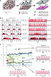
FIG. 1.

(A) Schematic of the local source node network architecture underlying mean field modeling. Excitatory (red circles) and inhibitory (black squares) neurons occupy a volume (left). Couplings are indicated by black connecting lines. Conceptually, both neuron types can be clustered in two subpopulations (middle). Each subpopulation can be then characterized by a mean behavior under certain conditions (right) and a mean connectivity (K11, K21, and K12) [Figure courtesy: Stefanescu and Jirsa (2008)]. (B) Effects of changing the coupling strength parameter K₁₁. Left: mainly, the excitatory coupling strength (n=0.5) leads to synchronization between neurons in the excitatory (red) and inhibitory subpopulations (black). Right: mainly inhibitory coupling: mainly, inhibitory coupling (n=1.5) leads to small oscillations in the inhibitory subpopulation and chaotic oscillations in the excitatory neurons [Figure courtesy: Stefanescu and Jirsa (2008)]. (C) Dynamical regimes of a dominantly inhibitory neural population: contour map of the mean-field amplitude calculated for a fixed ratio n=2.5 of inhibitory and excitatory coupling. Simulation databases are generated by sweeping values of n, K21/K11, K12, and σ and storing the resulting waveforms [Figure courtesy: Stefanescu and Jirsa (2008)].

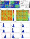
FIG. 2.

(A) Exemplary connectivity strength and distance matrices of a single subject obtained by diffusion tensor imaging tractography and directionality matrix of the macaque obtained from the CoCoMac database. Shown are normalized capacities between different source nodes that resemble the weight of individual node interactions estimated by the size of the fiber tract connecting the nodes (left) and distances between nodes (middle) estimated by the fiber-tract length between source node voxels. In addition, directionality information (black: explicit no connectivity) obtained from macaque axon-tract tracing data of the CoCoMac database is shown (right). Area names of the 96 regions are listed in Table 1—ordering of regions is equal in table and matrices. (B) Empirical and simulated functional connectivity (FC) of functional magnetic resonance imaging (fMRI) data. By a coarse numerical parameter space search, we identified parameter settings that yielded functional blood oxygen level-dependent (BOLD) connectivity that significantly correlated with the FC of empirical fMRI data (in the shown example, a correlation of r=0.47 has been achieved). The window length of the empirical BOLD data used to calculate FC was 38 scans=73,72 sec (repetition time=1.94 sec/sampling rate 0.5155 Hz). Altogether, the empirical BOLD data collected for a single subject had the length of 666 scans. We slid the window for the calculation of the BOLD FC over the entire empirical time series in steps of a single volume resulting in 666−38=628 different empirical FCs per subject. Simulated BOLD data were obtained by convolving a simulated mean field time series of the excitatory population (duration: 200 sec; sampled at 250 Hz) with the hemodynamic response function. This signal was subsequently downsampling to the fMRI scan frequency, resulting in a timeseries of 86 samples. Simulated FC was calculated over an identical time window of 38 scans as in empirical data. By sliding the window over the simulated time series in one-scan steps, we obtained 86−38=48 different simulated FCs. All simulated FCs were compared to all empirical FCs by calculating correlation coefficients resulting in 628×48=30,144 r values per subject and parameter setting. In this initial coarse parameter space search, we tested 78 different parameter settings by varying the parameters GC, structural connectivity (SC), v_cond, K11, K21, K12, and the six noise terms (abbreviations explained in Table 2). See examples for the distributions of resulting r-values in (C). The parameter values yielding the here-shown example of simulated data are listed in Table 2. The area names of the 96 regions for which FC is shown can be found in Table 1 in the identical order as depicted here. (C) Individual structure predicts function. BOLD FC matrices of nine subjects (represented by the different panels) were correlated with simulated FC matrices based on SC of a single subject. Shown are the distributions of correlation coefficients (CCs) for 30,144 comparisons (628 empirical FCs×48 simulated FCs). The red-boxed panel contains the data where SC and FC come from same subject—resulting in notably higher CCs.

FIG. 3.

(A) Exemplary local field source activity of two different nodes. Left: Fifteen seconds of local mean field activity. Middle: Power spectra. While in the upper panel we see dominant alpha-oscillations, the source in the lower panel exhibits a dominant delta-activity. Right: Topography of the alpha- and delta-rhythms. (B) Simulated electroencephalography (EEG). Displayed are 15 sec of approximated EEG activity for six selected channels referenced to channel FCz. (C) BOLD timeseries of regions of interest (ROIs) exhibiting high FC (top row) and low FC (bottom row). Left: Simulated BOLD signal. Right: Empirical BOLD signal. Timecourses of identical ROIs are shown for empirical and simulated data. (D) Frequency spectra of mean-field source activity, EEG, and BOLD signals of exemplary nodes/channels. Note the peaks in the delta-/alpha-range for the electrophysiological simulations and in the <0.1-Hz range for BOLD.

FIG. 4.

EEG forward modeling—calculating the EEG channel signals yielded by the neuronal source activity at the cortical nodes. (A) Triangulation of the Montreal Neurological Institute brain surface constructed by 81,920 vertices. The regions representing the cortical and subcortical nodes are color coded. In this example, the large-scale model comprises 96 regions; however, 14 of them representing subcortical structures that do not directly contribute to the channel space signals and therefore represented by a single color here. (B) The vertex normals represent the orientation of the dipoles and serve for the calculation of the lead field matrix that describes the transformation from the signals at the cortical sources to the EEG channel space.

FIG. 5.

Exemplary motif-fitting results. Shown are one-second snippets of source estimates from EEG (red) and corresponding model fits (blue). Parameters were obtained using a random Monte Carlo search routine that optimized waveform correlation after running for one hour on a single core of a 2.13-GHz Intel Core 2 Duo processor. Despite high correlation coefficients (r=0.78 for the best fit), some waveform features were not captured appropriately. We expect more sophisticated parameter estimation approaches (cf. section A, choice of parameter estimation algorithms) to produce even better fits.

FIG. 6.

Model-based knowledge generation. The virtual brain estimates parameter sets that enable the model-based replication of short empirical source activity timeseries. Upon emulation of observable timeseries, internal model state variables can then be analyzed to infer knowledge about unobservable system states. Empirical EEG and BOLD data are used to estimate electrical source activity. Employing individual structural priors (fiber-tract capacities and distances), each node's activity can be disentangled from the influences of the other nodes. Spatial and temporal properties of the resulting data are compared to the model output. Parameter settings yielding the best fit are identified. A central point is the identification of spatiotemporal motifs, that is, the identification of similar dynamical behaviors in simulated and empirical data. Matching empirical- and model-based structural flows on manifolds are stored in a dictionary, for example, in the form of prototypical source timecourses. Priors, that is, initial parameter settings known to yield specific classes of dynamics observed in empirical data, are taken from the dictionary for subsequent simulations. Taking advantage from the pool of existing knowledge increasingly reduces the costs for parameter optimization for different empirical dynamical scenarios. In other words, an integrative method of induction and deduction serves our model optimization procedure. Statistical analysis of the parameters sets stored in the dictionary yields the desired insight about which biophysical and/or mathematical settings are related to the different observed brain states.

FIG. 7.

Simulated FC of individual frequency bands of mean-field activity and its correlation with the empirical BOLD FC are shown in Figure 2B. Area names of the 96 regions are listed in Table 1—ordering of regions is equal in table and matrices.

References

1. Agrafiotis DK. Stochastic proximity embedding. J Comput Chem. 2003;24:1215–1221. - PubMed
1. Amari S.-i. “Dynamics of pattern formation in lateral-inhibition type neural fields.”. Biological cybernetics. 1977;27:77–87. - PubMed
1. Aquino KM. Schira MM, et al. Hemodynamic traveling waves in human visual cortex. PLoS Comput Biol. 2012;8:e1002435. - PMC - PubMed
1. Assisi CG. Jirsa VK, et al. Synchrony and clustering in heterogeneous networks with global coupling and parameter dispersion. Phys Rev Lett. 2005;94:018106. - PubMed
1. Attwell D. Iadecola C. The neural basis of functional brain imaging signals. Trends Neurosci. 2002;25:621–625. - PubMed
Publication types