. 2013 Jun;32(6):1033-42.
doi: 10.1109/TMI.2013.2248163. Epub 2013 Feb 21.

Comparison of Kasai autocorrelation and maximum likelihood estimators for Doppler optical coherence tomography

Affiliations

Comparison of Kasai autocorrelation and maximum likelihood estimators for Doppler optical coherence tomography

Aaron C Chan et al. IEEE Trans Med Imaging. 2013 Jun.

Abstract

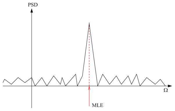
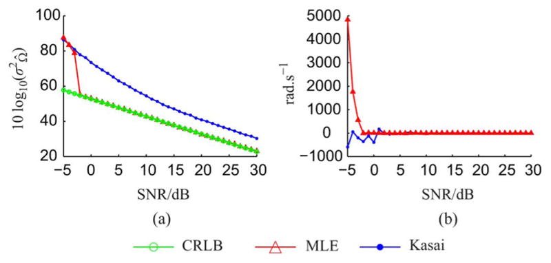
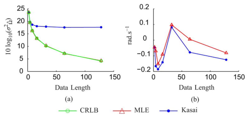
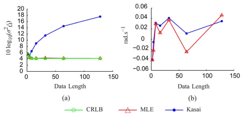
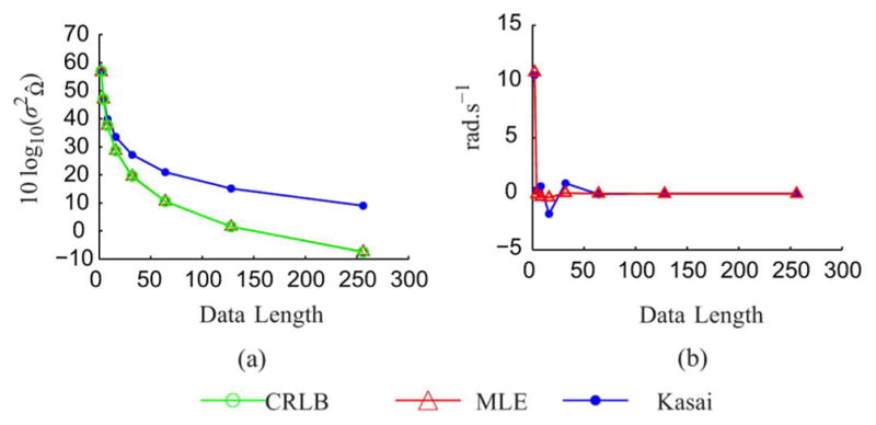
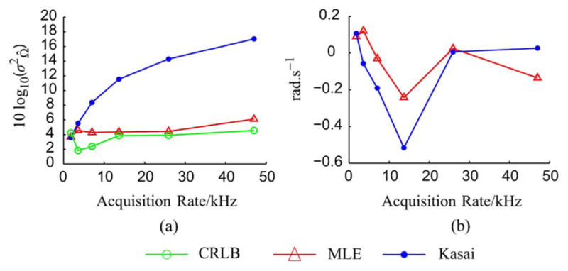
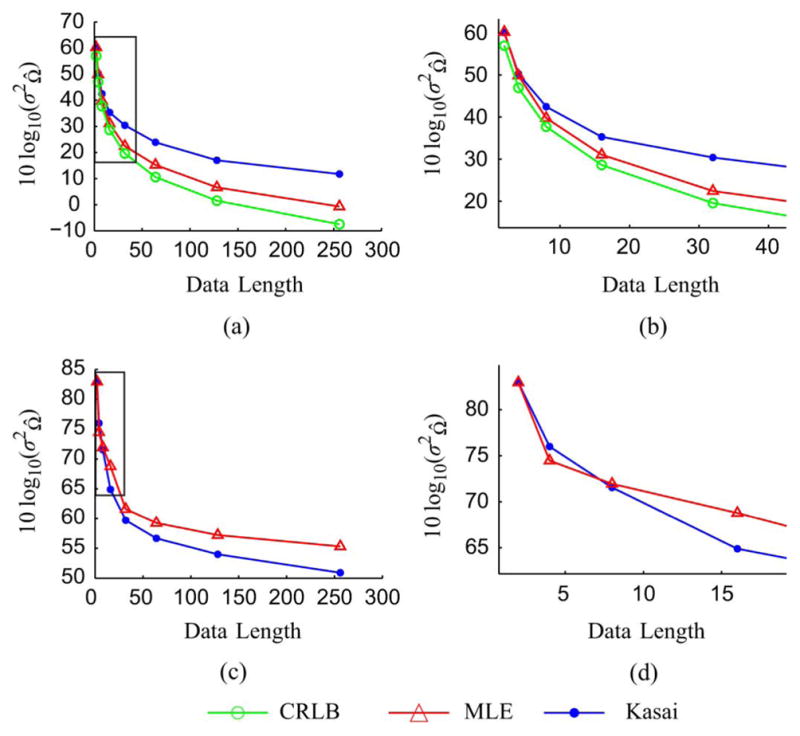
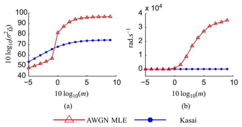
In optical coherence tomography (OCT) and ultrasound, unbiased Doppler frequency estimators with low variance are desirable for blood velocity estimation. Hardware improvements in OCT mean that ever higher acquisition rates are possible, which should also, in principle, improve estimation performance. Paradoxically, however, the widely used Kasai autocorrelation estimator's performance worsens with increasing acquisition rate. We propose that parametric estimators based on accurate models of noise statistics can offer better performance. We derive a maximum likelihood estimator (MLE) based on a simple additive white Gaussian noise model, and show that it can outperform the Kasai autocorrelation estimator. In addition, we also derive the Cramer Rao lower bound (CRLB), and show that the variance of the MLE approaches the CRLB for moderate data lengths and noise levels. We note that the MLE performance improves with longer acquisition time, and remains constant or improves with higher acquisition rates. These qualities may make it a preferred technique as OCT imaging speed continues to improve. Finally, our work motivates the development of more general parametric estimators based on statistical models of decorrelation noise.


Figures

Fig. 1
Fig. 1
MLE for Doppler frequency is the location of the peak of the power spectral density.
Fig. 2
Fig. 2
(a) The sample variance of estimates (simulated) compared with the CRLB, for N = 32, T = 0.001 s. The y-axis is the estimator variance in decibels. The variance of the MLE can be seen to rapidly approach the bound even at low SNRs. The Kasai estimator is more than 7 dB worse than the MLE, even at high SNRs. (b) Estimator bias in radians per second with SNR. For moderate SNRs, these values are too small to be significant, hence the estimator variance and the MSE can be considered to be the same.
Fig. 3
Fig. 3
(a) Variance of Kasai and ML estimators (simulated) against data length (varying acquisition rate), for T = 0.002 s at a constant SNR of 36.5 dB. In practice, holding the SNR constant would require increasing the detected photon rate (power) with increasing acquisition rate. The acquisition rates used were 20, 21, …, 26 kHz. The Kasai estimator performance does not improve significantly with data length. The MLE performance improves with data length and closely matches the CRLB. (b) Bias estimates for Kasai estimator and MLE suggest that at 36.5 dB SNR, both are unbiased.
Fig. 4
Fig. 4
(a) Variance of Kasai and ML estimators (simulated) with shot noise SNR scaling for T = 0.002 s against data length (varying acquisition rate). This corresponds to maintaining a constant detected photon rate (power) with increasing acquisition rate. The SNRs for N = 2, 4, …, 128 were 54.6, 51.6, 48.6, 45.6, 42.6, 39.5, and 36.5, respectively, approximating the experimental values encountered in Fig. 6 and Table II. The acquisition rates were 20,21, …, 26 kHz. The SNR scales as T/N, hence the CRLB is constant with data length, as shown in (21). The Kasai estimator performance deteriorates with increasing sampling rate. (b) Bias estimates for Kasai estimator and MLE suggest that, both are unbiased.
Fig. 5
Fig. 5
(a) Variance of Kasai and ML estimators against data length (varying acquisition time), for a constant acquisition rate of 47 kHz at an SNR of 36.5 dB. Compare these simulated data with Fig. 7. As the acquisition time is increased, both estimator variances and the CRLB are reduced. The MLE performance closely matches that of the CRLB. (b) Bias estimates for Kasai estimator and MLE suggest that both are unbiased.
Fig. 6
Fig. 6
(a) Plot of experimentally determined estimator performance against acquisition rate from a fixed M-scan of a nonmoving cover-glass, estimated from 100 samples, with T ≈ 0.0025 s. The SNRs (see Table II) were estimated from data and used to determine the CRLB. The experimentally measured SNR was 36.5 dB for an acquisition rate of 47 kHz. These results are in agreement with Fig. 4, taking into account a longer acquisition time. (b) The bias estimates are on the order of tenths of rad.s−1, which is negligible and the estimators can be assumed to be unbiased.
Fig. 7
Fig. 7
(a), (b) Experimental verification of the Kasai and ML estimator variances against data length (acquisition time), for constant acquisition rate of 47 kHz measured on the surface of a cover-glass. The CRLB was plotted assuming a 36.5 dB SNR. Compare this figure with Fig. 5(a). The MLE slowly diverges from the CRLB as acquisition times increase, contrary to the prediction from simulation, due to other sources of noise. (c), (d) Verification using a 0.1 ml.hr−1 intralipid flow phantom, at about one quarter in from the edge of the tubing. The SNR was approximately 10.0 dB. The MLE performs better than the Kasai estimator for data lengths of up to 8 or acquisition times of up to 0.17 ms. For data lengths longer than this, decorrelation noise becomes significant and the MLE performance becomes worse.
Fig. 8
Fig. 8
Color Doppler maps, with dimensions of 512 by 100, generated using the Kasai [(a), (b)] and AWGN ML [(c), (d)] estimators. The flow rate was 0.1 ml.hr−1, using intralipid-10% at a 16° incline, with a 10 dB SNR. Scanning was done at a fixed location. The x-axis is a time axis. The line scan rate was 47 kHz, and estimates were made with 4 [(a), (c)] and 16 [(b), (d)] data points, respectively, corresponding to acquisition times of 0.09 and 0.34 ms. These represent two of the conditions shown in Fig. 7(c) and (d). The variances of the Kasai estimator were 4.02 × 10⁷ rad2.s−2 (76.0 dB) and 3.12 × 10⁶ rad2.s−2 (64.9 dB), respectively. For the MLE, zero padding was used to increase the FFT lengths by 256. For acquisition times of roughly 0.17 ms and below the MLE outperforms the Kasai estimator. The variances of the ML estimates were 2.83 × 10⁷ rad2.s−2 (74.5 dB) and 7.63 × 10⁶ rad2.s−2 (68.8 dB), respectively.
Fig. 9
Fig. 9
(a) The sample variance of estimates for varying degrees of multiplicative noise with no additive noise for, N = 32, T = 0.001 s. The x-axis shows the ratio of multiplicative noise components to signal components in decibels. At roughly −0.5 dB the estimators have equal performance. (b) Estimator bias in radians per second with SNR.

Similar articles

Cited by

References

    1. Izatt JA, Kulkarni MD, Yazdanfar S, Barton JK, Welch AJ. In vivo bidirectional color Doppler flow imaging of picoliter blood volumes using optical coherence tomography. Opt Lett. 1997 Sep;22(18):1439–1441. - PubMed
    1. Chen Z, Milner TE, Dave D, Nelson JS. Optical Doppler tomographic imaging of fluid flow velocity in highly scattering media. Opt Lett. 1997 Jan;22(1):64–66. - PubMed
    1. Srinivasan VJ, Sakadzic S, Gorczynska I, Ruvinskaya S, Wu W, Fujimoto JG, Boas DA. Quantitative cerebral blood flow with optical coherence tomography. Opt Exp. 2010 Feb;18(3):2477–2494. - PMC - PubMed
    1. Nezam SMM, Joo C, Tearney GJ, de Boer JF. Application of maximum likelihood estimator in nano-scale optical path length measurement using spectral-domain optical coherence phase microscopy. Opt Exp. 2008 Oct;16(22):17186–17195. - PMC - PubMed
    1. Szkulmowski M, Szkulmowska A, Bajraszewski T, Kowalczyk A, Wojtkowski M. Flow velocity estimation using joint spectral and time domain optical coherence tomography. Opt Exp. 2008 Apr;16(9):6008–6025. - PubMed

Publication types

MeSH terms