Neural integrators for decision making: a favorable tradeoff between robustness and sensitivity

Abstract

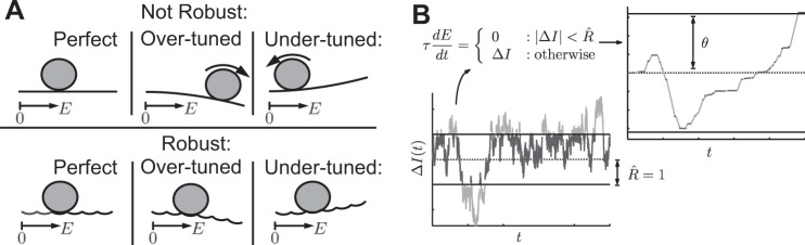
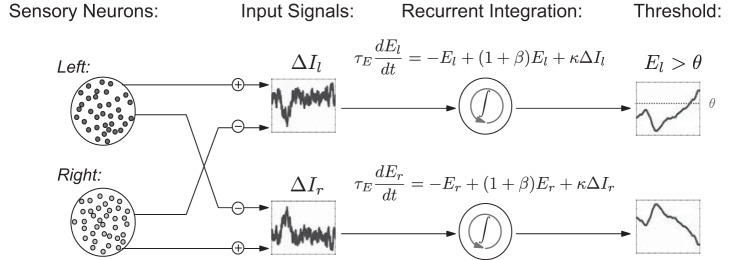
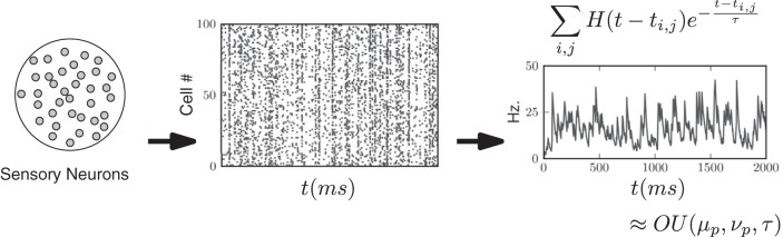
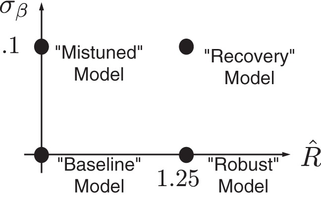
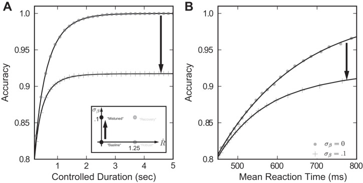
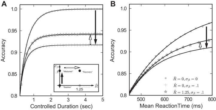
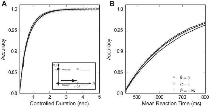
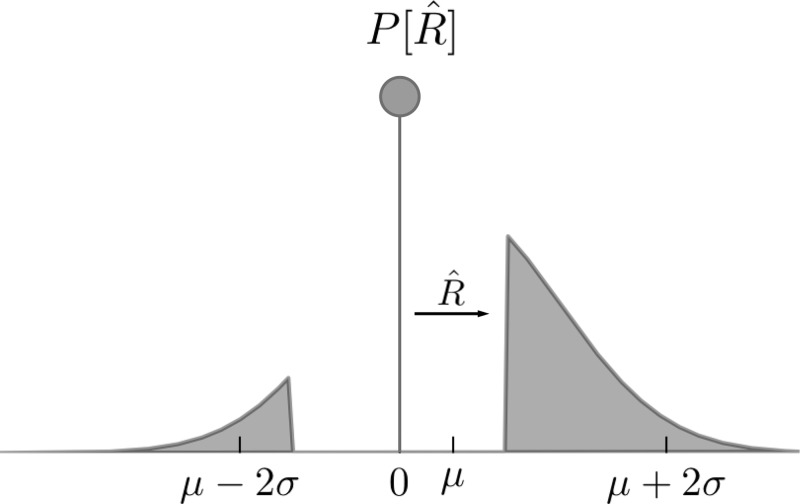
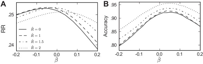
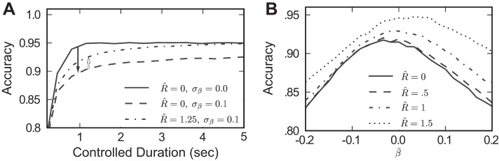
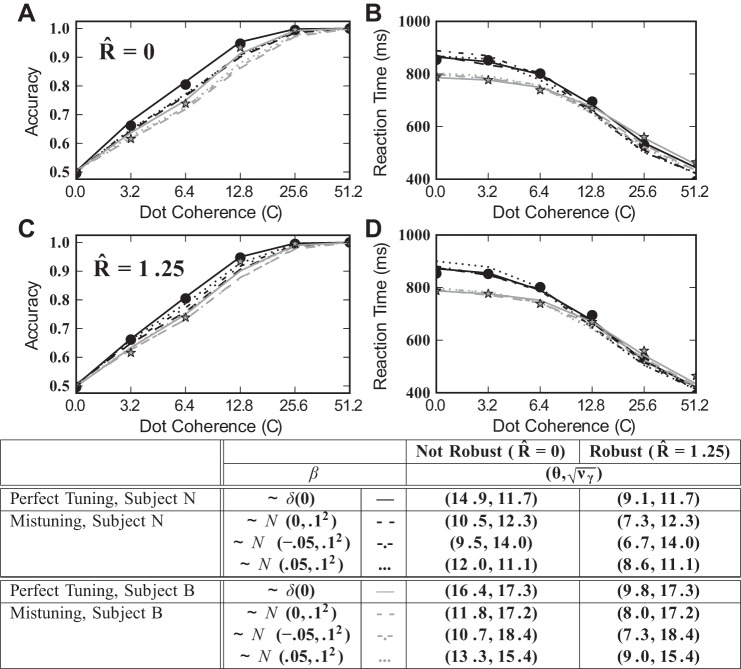
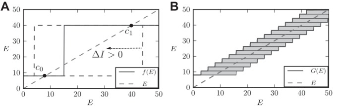
A key step in many perceptual decision tasks is the integration of sensory inputs over time, but a fundamental questions remain about how this is accomplished in neural circuits. One possibility is to balance decay modes of membranes and synapses with recurrent excitation. To allow integration over long timescales, however, this balance must be exceedingly precise. The need for fine tuning can be overcome via a "robust integrator" mechanism in which momentary inputs must be above a preset limit to be registered by the circuit. The degree of this limiting embodies a tradeoff between sensitivity to the input stream and robustness against parameter mistuning. Here, we analyze the consequences of this tradeoff for decision-making performance. For concreteness, we focus on the well-studied random dot motion discrimination task and constrain stimulus parameters by experimental data. We show that mistuning feedback in an integrator circuit decreases decision performance but that the robust integrator mechanism can limit this loss. Intriguingly, even for perfectly tuned circuits with no immediate need for a robustness mechanism, including one often does not impose a substantial penalty for decision-making performance. The implication is that robust integrators may be well suited to subserve the basic function of evidence integration in many cognitive tasks. We develop these ideas using simulations of coupled neural units and the mathematics of sequential analysis.

Keywords: decision making; neural integrator.

Fig. 1.

Schematic of neural integrator models. A: visualizing integration via an energy surface (Pouget and Latham 2002; Goldman et al. 2009). The robust integrator can “fixate” at a range of discrete values, indicated by a sequence of potential wells, despite mistuning of circuit feedback. These wells can be arbitrarily “close” in the energy landscape, providing a mechanism for graded persistent activity. Without these wells (the nonrobust case), activity in a mistuned integrator would either exponentially grow or decay, as at top. Perturbing the robust integrator from one well to the next, however, requires sufficiently strong momentary input. B: as a consequence, low-amplitude segments in the input signal ΔI(t), below a robustness limit R, are not accumulated by a robust integrator: only the high-amplitude segments are. The piecewise definition of Eq. 5 captures this robustness behavior, resulting in the accumulated activity shown, and may be related to, e.g., a detailed bistable-subpopulation model. A decision is expressed when the accumulated value E(t) crosses the decision threshold θ.

Fig. 2.

Overview of model. Simulations of sensory neurons and neural recordings are used to define the left and right inputs ΔI_l(t) and ΔI_r(t) to neural integrators. These inputs are modeled by Gaussian [Ornstein-Uhlenbeck (OU)] processes, which capture noise in the encoding of the motion strength by each pool of spiking neurons (see Eqs. 1–3 for definition of input signals). Similar to Mazurek et al. (2003), the activity levels of the left and right integrators E_l(t) and E_r(t) encode accumulated evidence for each alternative. In the reaction time task, E_l(t) and E_r(t) race to thresholds to determine choice on each trial. In the controlled duration task, the choice is made in favor of the integrator with higher activity at the end of the stimulus presentation.

Fig. 3.

Construction of Gaussian (OU) processes to represent fluctuating, trial-by-trial firing rate of a pool of weakly correlated MT neurons (Bair et al. 2001; Zohary et al. 1994). As in Mazurek and Shadlen (2002), these motion sensitive neurons provide direct input to our model integrator circuits. Simulated spike trains from weakly correlated, direction selective pools of neurons are shown as a rastergram. All spikes before time t, a sum over the jth spike from the ith neuron, for all i and j, are convolved with an exponential filter, and then summed to create a continuous stochastic output (right); here, H(t) is the Heaviside function. We approximated this output by a simpler Gaussian (OU) process to simplify numerical and analytical computations that follow.

Fig. 4.

Parameter space view of 4 integrator models, with different values of the robustness limit R̂ and feedback mistuning variability σ_β. The impact of transitioning from one model to another by changing parameters is either to enhance or diminish performance or to have a neutral effect (see text).

Fig. 5.

Mistuned feedback diminishes decision performance. Inset: plots depict a move in parameter space from the baseline model to the mistuned model by changing σ_β = 0 → 0:1. In this and subsequent plots, simulation results are given with markers; lines are rational polynomial fits. A: in the controlled duration task, accuracy is lower for the mistuned model than for the baseline model at every trial duration, indicating a loss of performance when σ_β increases. B: in the reaction time task, we parametrically plot all [reaction time (RT), accuracy] pairs attained by varying the decision threshold θ. Once again, accuracy is diminished by mistuning for a fixed mean reaction time.

Fig. 6.

Increasing the robustness limit R̂ helps recover performance lost due to feedback mistuning. Results of simulation are plotted with fitting lines. Inset: we illustrate this by moving in parameter space from the mistuned model to the recovery model, by changing R̂ = 0 → 1.25. The impact on decision performance is shown for both the controlled duration (A) and reaction time (B) tasks. We find that R̂ > 0 yields a performance gain for the recovery model compared with the mistuned model (i.e., for a fixed accuracy, mean reaction time is increased).

Fig. 7.

Increasing R̂ alone does not compromise performance. Only simulation results, without fitting lines, are plotted for clarity. Inset: we illustrate this by moving in parameter space directly from the baseline to the “robust” model. For both controlled duration (A) and reaction time tasks (B), we plot the relationship between mean reaction time and accuracy. Circles give results for the baseline model, and “x” and “y” markers for the robust model at R̂ = 1 and 1.25, respectively. These curves are very similar in the baseline case, indicating little change in decision performance due to the robustness limit R̂ = 1.25.

Fig. 8.

R̂ affects the discrete time increment distribution. The probability density function of the random variable Z_R̂, with probability mass for values between the robustness limit R̂ reallocated as a delta function centered at zero (in this figure, R̂ = 1).

Fig. 9.

Accuracy of the discrete/independent and continuous/correlated models for the controlled duration task, T = 500 ms. A: approximation of the performance of the continuous/correlated model via Eq. 15 is plotted as a black curve, and that predicted by the discrete/independent model with identical signal increments is plotted as a gray curve. B: disparity in performance of these 2 models can be partially understood by observing the decorrelating effect of R̂ on the autocorrelation function for the evidence stream in the continuous/correlated model. Inset: 2 of these same functions (for R̂ = 0 and R̂ = 1.5) are plotted normalized to their peak value.

Fig. 10.

Distribution of 2 neighboring (in time) samples of the incoming signal. A: before application of the robustness operation, the samples Z(t₁) and Z(t₂) covary with correlation coefficient Corr = 0:5. B: after applying robustness (R̂ = 1), samples with Z(t₁) < R̂ are mapped to Z_R̂ (t₁) = 0, and likewise for samples with Z(t₂) < R̂. As a consequence, samples covary less in the region where either sample has been thresholded to zero, yielding Corr = 0:42.

Fig. 11.

In the discrete model R̂ increases RT but not accuracy. A: the second real root h₀ of M_ZR̂(s) remains unchanged as R̂ increases from 0 → 2 (lines are uniformly distributed in this range). This implies that in the reaction time task, no changes in the accuracy will be observed (see Eq. 16). B: however, the speed accuracy tradeoff will be affected, once E[Ẑ_R] begins to diminish (see Eq. 17). This performance loss begins for R̂ > 0.5, in contrast to the performance of the continuous time model (see Fig. 7B).

Fig. 12.

Robustness improves reward rate (RR) under mistuning. A: speed accuracy curves plotted for multiple values of R̂; as in previous figures, the greater accuracies found at fixed mean reaction times indicate that performance improves as R̂ increases. The heavy line indicates the baseline case of a perfectly tuned, nonrobust integrator (repeated from Fig. 5B). RR level curves are plotted in background (dotted lines; see text), and points along speed accuracy curves that maximize RR are shown as circles. These maximal values of RR are plotted in B, demonstrating the nonmonotonic relationship between R̂ and the best achievable RR.

Fig. 13.

Robustness improves performance across a range of mistuning biases β̄. In both the reaction time (A) and controlled duration (B) tasks, robustness helps improve performance when β ∼ N (β̄, 0.1²), for all values of β̄ shown. As in previous figures, the coherence of the sensory input is C = 12.8. In the reaction time task (A), θ is varied for each value of β̄ to find the maximal possible RR, and performance gains are largest for β̄ > 0. In the controlled duration task, substantial gains are possible across the range of β̄ values.

Fig. 14.

Effect of the robustness limit R̂ on decision performance in a controlled duration task, under the bounded integration model of Kiani et al. (2008). Dot coherence C = 12.8. A: increasing the robustness limit R̂ helps recover performance lost to mistuning at multiple reaction times in the controlled duration task. Specifically, moving from the baseline model to the mistuned model decreases decision accuracy, but this lost accuracy can be partially or fully recovered for R̂ > 0. B: when allowing for biased mistuning (β̄ ≠ 0, σ = 0.1), R̂ still allows for recovery of performance; effects are most pronounced when β̄ > 0.

Fig. 15.

Accuracy (A and C) and chronometric (B and D) functions: data and model predictions. Solid dots and stars are behavioral data for a rhesus monkey [subject “N” and “B,” respectively (Roitman and Shadlen 2002)]. In A–D, the accuracy and chronometric functions are fit to behavioral data via least squares, over the free parameters θ and ν_γ. In A and B, the robustness threshold R̂ = 0, and results are shown for baseline and exemplar mistuned models (see legend in table). In C and D, results are shown for the robust and recovery models (R is fixed across the range of coherence values so that R̂ = 1.25 at C = 0). The close matches to data points indicate that these models can be reconciled with the psychophysical performance of individual subjects by varying few parameters. Parameter values for each curve are summarized in the table.

Fig. A1.

Simultaneous plots of the identity line and the feedback line, G(Ê), for 2 circuits with differing numbers of subunits. A: here N = 1, and so the feedback line G(Ê) = f(Ê) is exactly determined as a function of Ê = r₁ (see Eq. 25). The 2 intersections c₀ and c₁ are stable fixed points. In this way, the subunit firing rate is bistable, and the value attained will depend on the history of the circuit activity. As ΔI is changed, this translates f(Ê); eventually eliminating either c₀ or c₁ and forcing the subunit to the remaining stable fixed point (here, c₀ corresponds to Ê = 8 Hz. and c₁ to 40 Hz). In dashed curves, the feedback line is plotted for 2 such values of ΔI. B: now N > 1 and so the feedback line G(Ê) is no longer unambiguously specified as a function of its argument. The function is instead the sum of N potentially bivalued functions, whose actual values will depend on the stimulus history. We represent this fact by plotting the feedback line as a set of stacked boxes, representing the potential contribution of the ith subunit to the total integrator dynamics (Goldman et al. 2003).

Fig. A2.

Plot of possible equilibria for Eq. 24. A: extent of each multivalued feedback function defines the minimum input necessary to perturb the system away from equilibrium, defining the fixation lines. As N → ∞, the stable fixed points become more tightly packed on the interval (r⁻; r⁺). B: when the integrator is mistuned, the fixation lines and the feedback line are no longer parallel. The rate that the integrator accumulates input is approximated by the distance between the center line of the feedback subunits [G̃(Ê)], and the feedback line. However, integration only occurs when the “fixation condition” is no longer satisfied, i.e., when the feedback line is no longer bounded by the fixation lines at the current value of Ê.

Fig. A3.

Comparison of integration by Eqs. 22 and 5, R̂ = 0.1 (A), R̂ = 0.5 (B), and R̂ = 11 (C). Histograms of the relative error between the values of E(t) and Ê(t) at t = 500 ms are plotted as insets (see Eq. 36). Means and SD (μ, σ) for each distribution are, respectively, (0.0097, 0.022), (0.0183, 0.0453), and (0.1342, 0.1358). At these levels of R̂, E approximates Ê low to moderate error.

Fig. A4.

Performance comparison of 2 models of robust integration, reaction time task. In each panel, the lines are the same as in Fig. 6 legend. Downward arrows indicates the impact of mistuning: increasing σ_γ from 0 to 0.1. Upward arrows show the effect of robustness: increasing R̂ from 0 to 1.25. Overall, we see that robustness has an even greater positive impact on the performance of the circuit-based model (here q = 1, r⁻ = 0, r⁺ = 50, N = 250, κ = 1/9; p is then adjusted to give the required robustness level). Data were generated from 50,000 numerical trials per value.

References

1. Averbeck B, Latham P, Pouget A. Neural correlations, population coding and computation. Nat Rev Neurosci 7: 358–366, 2006 - PubMed
1. Bair W, Zohary E, Newsome WT. Correlated firing in macaque visual area MT: time scales and relationship to behavior. J Neurosci 21: 1676–1697, 2001 - PMC - PubMed
1. Billingsley P. Probability and Measure. Hoboken, NJ: Wiley-Interscience, 1986
1. Bogacz R, Brown E, Holmes P, Cohen JD. The physics of optimal decision making: a formal analysis of models of performance in two-alternative forced-choice tasks. Psychol Rev 113: 700–765, 2006 - PubMed
1. Britten KH, Shadlen MN, Newsome WT, Movshon JA. The analysis of visual motion: a comparison of neuronal and psychophysical performance. J Neurosci 12: 4745–4765, 1992 - PMC - PubMed
Publication types
LinkOut - more resources