The sparseness of mixed selectivity neurons controls the generalization-discrimination trade-off

Abstract

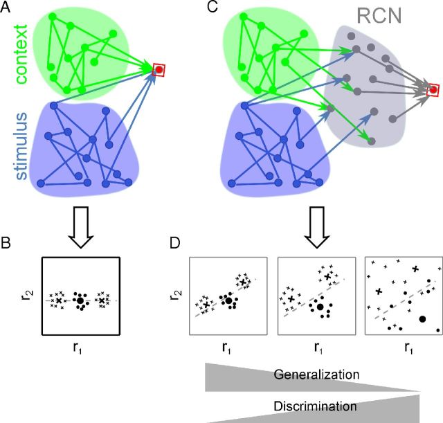
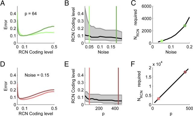
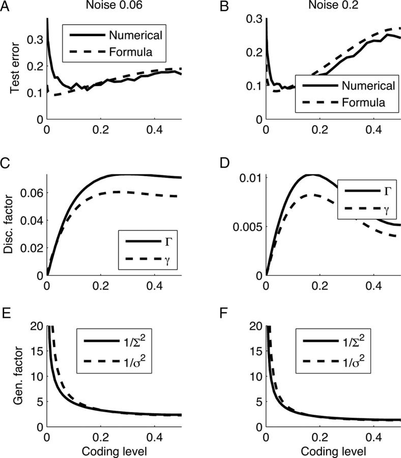
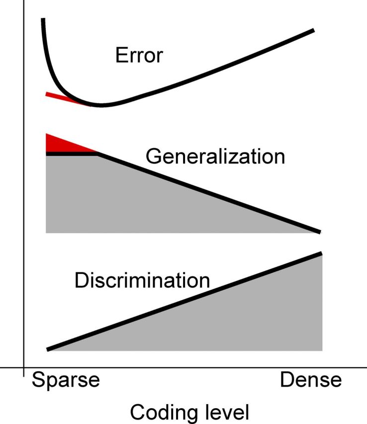
Intelligent behavior requires integrating several sources of information in a meaningful fashion-be it context with stimulus or shape with color and size. This requires the underlying neural mechanism to respond in a different manner to similar inputs (discrimination), while maintaining a consistent response for noisy variations of the same input (generalization). We show that neurons that mix information sources via random connectivity can form an easy to read representation of input combinations. Using analytical and numerical tools, we show that the coding level or sparseness of these neurons' activity controls a trade-off between generalization and discrimination, with the optimal level depending on the task at hand. In all realistic situations that we analyzed, the optimal fraction of inputs to which a neuron responds is close to 0.1. Finally, we predict a relation between a measurable property of the neural representation and task performance.

Figure 1.

The challenge of integrating sources of information in the presence of noise. A, A single neuron (red) receiving input from two sources (green and blue, representing for instance a sensory stimulus and the context in which it appears). B, Representations in the input space that are not linearly separable (typical situation when multiple sources of information are integrated). The axes of the plane represent independent patterns of activity of the input neurons, for instance the firing rate of two different neurons. Each point on the plane represents a different input activity pattern, and the symbols represent how patterns should be classified. For example, crosses are inputs that should activate the readout neuron, and circles are inputs that should inactivate it. The inputs to be classified are constructed as noisy variations of three prototypes (large symbols) that represent three different classes. In this example, the correlations between the inputs constrain the large symbols to lie on a line, making the classification problem linearly nonseparable (i.e., there is no single line separating the crosses from the circles). C, An intermediate layer of randomly connected neurons, RCNs, solves the linear separability problem. D, Neural representations in the RCN space for three different transformations performed by the RCNs on the input space. The axes now represent the activity of two RCNs. For all the transformations, the dimensionality of the inputs increases (the prototypes spread out on a plane), aiding discrimination (distance between large symbols). But too much decorrelation (right) can amplify noise and degrade the generalization ability (dispersion of small symbols). The sparseness or the coding level of the RCNs mediates this generalization–discrimination tradeoff.

Figure 2.

Segregated representations are not linearly separable. A, Two sources of N neurons each are each in one of two configurations (A,B for the first source, C,D for the second one), and they are read out by a linear classifier. B, The four possible input patterns in a 2N dimensional space. C, Despite being 2N dimensional, the four patterns are actually on a 2D plane due to their structure. Four points on a 2D plane cannot be arbitrarily classified (e.g., AD and BC cannot be separated from AC and BD). The spatial arrangement of the four points is a consequence of the correlations between all the patterns (e.g., AC has a large overlap or correlation with AD, as the first source is in the same state). D, For more than four patterns, the gap between the number of patterns and their corresponding dimension increases, impairing linear separability. The three curves show the number of dimensions versus the number (Num.) of inputs to be classified for two input sources with 5, 10, or 15 states each (p = 25, 100, or 225 possible patterns). E, Classification errors arise when there are more patterns than dimensions, even when only a subset of possible patterns is used. The graph shows that the fraction of correctly classified patterns drops rapidly once the number of patterns used exceeds the input dimensionality (compare to D).

Figure 3.

RCNs enable linear separability by increasing input dimensionality. A, The dimensionality of the representation in RCN space as a function of the number of RCNs for 64 patterns (two sources of eight states each). For dense representations, every RCN increases the dimensionality by 1, while for sparse ones this slope is smaller. Correct classification requires a high enough dimensionality, and the black markers denote the point where 95% of the patterns could be classified correctly. Sparseness is measured by f, the fraction of patterns that activate a given RCN. B, Similar to A, but for 225 patterns. Note that the detrimental effect of sparse coding is reduced. C, The ordinate denotes the minimum number of RCNs required to classify 80% of the patterns correctly normalized by the number of patterns considered. Note that as the number of patterns (and thereby RCNs) increases, sparser representations become more efficient. For each number of patterns there is a critical (Crit.) coding level (f_crit) below which performance deteriorates (green dotted line; see Materials and Methods). D, This coding level scales as a power law of the number of patterns with an exponent of approximately −0.8.

Figure 4.

RCN coding level shifts the balance between discrimination and generalization. A, Neural architecture, as in Figure 1C. The crosses and circles represent the patterns to be classified, as in Figure 1D. The original segregated representations are nonlinearly separable for a classification problem analogous to the exclusive OR (opposite points should produce the same output). The RCNs increase the dimensionality, making the problem linearly separable (now a plane can separate crosses from circles). B, Transformation of Hamming distances in the RCN space for two coding levels (blue, 0.5; red, 0.1). The distance in the RCN space is plotted versus the distance in the input space. Although distances are distorted, their ranking is preserved (e.g., small distances map to small distances). C–F, How generalization and discrimination abilities vary with the coding level of RCN representations. C, The generalization ability is estimated as the fraction of RCNs that respond in a consistent manner to noisy realizations of the same input (n = 0.1). The shaded area represents the distribution of input currents to different RCNs for a particular input pattern (A, C, for the two sources, respectively). For dense representations (blue, threshold at zero) there is a larger fraction of RCNs that is around the activation threshold compared to the sparse case. D, The fraction of consistent RCNs decreases with coding level. E, The discrimination ability is estimated as the fraction of RCNs that respond differentially to a pair of patterns, differing only by the state of one source. The gray area represents the distribution of the currents to the RCNs for AC and AD inputs (differing in the second source). The area of colored shading represents the fraction of RCNs that respond differentially to the two combinations of inputs (for one input the current is positive and for the other it is negative). F, Discrimination increases with coding level.

Figure 5.

The optimal coding level is ∼10%. A, The dependence of classification error on RCN coding level for two different noise levels: n = 0.05 (light) and n = 0.175 (dark). Two sources of eight states each were used. B, Extension of A for many noise levels, showing the dependence of the optimal coding level (black curve) on the input noise. The sensitivity of the error to coding level is indicated by shading those coding levels that result in an error up to 20% worse than the optimal one. The colored lines denote the values used in A. C, The number of RCNs required to maintain the minimal error at roughly 0.1 (i.e., 10% of the patterns misclassified). D–F, Similar to the panels in the top row, but varying the number of patterns. Patterns were generated by two input sources with identical numbers of states. The two parameter values shown are p = 81 (light) and p = 441 (dark).

Figure 6.

Measuring the discrimination (γ) and generalization (1/σ²) factors from neural data (simulated data). The rasters show the spikes of a single hypothetical neuron in response to several presentations of four combinations of stimuli (A/B) and contexts (C/D). The mean firing rates for each combination of input sources are calculated (bars below the rasters). The squared differences of firing rates are averaged for two cases: inputs differing by either stimulus or context, but not both (left cluster of arrows that point to the two dashed lines that correspond to these pairs, Δ₁), and inputs differing in both stimulus and context (right cluster, Δ₂). The green error bars denote the trial to trial variability used to compute σ². Inset, γ is a measure of the nonlinearity in the transformation to RCN space. In the input space, the difference between pairs of inputs belonging to Δ₁ is half the difference between pairs belonging to Δ₂. The factor γ measures the deviation from this relation in RCN space.

Figure 7.

Estimating error from experimentally accessible factors versus the actual error. The figure shows the ratio between the error obtained using either dense (A, f = 0.5) or ultra-sparse (B, f = 0.01) to that obtained using sparse (f = 0.1) coding. Ratios are shown for various levels of the input noise. The x-axis shows the ratio derived from the full simulation, while the y-axis is computed using the formula and calculating γ and σ² from 30 trials of 100 RCNs. The color bar shows the noise level (same values as in Fig. 5A–C, using 64 patterns).

Figure 8.

Components of generalization discrimination tradeoff. A, B, Comparing the actual test error with the one predicted by Equation 20. Note the discrepancy in sparse coding levels, which is caused mainly by the small denominator of Equation 20. C, D, Discrimination factor, exact Γ and approximate γ, as a function of coding level. E, F, Generalization factor, exact 1/Σ² and approximate 1/σ², as a function of coding level. All values were derived using 64 input patterns and 424 (4227) RCNs for 0.06 (0.2) noise.

Figure 9.

Summarizing our understanding of the generalization discrimination trade-off. Dense coding is optimal for discriminating between similar inputs but has a detrimental effect on the ability to generalize. Decreasing coding level shifts this balance and improves the overall classification ability, but for very sparse coding levels (f < 0.1) finite size effects limit the generalization ability, and thus the classification error increases. In the limit of very large neural systems (red lines), the classification error would keep increasing as the representations become sparser, and this would compensate for the decrease in the ability to discriminate.

References

1. Amit DJ, Fusi S. Learning in neural networks with material synapses. Neural Comput. 1994;6:957–982.
1. Asaad WF, Rainer G, Miller EK. Neural activity in the primate prefrontal cortex during associative learning. Neuron. 1998;21:1399–1407. - PubMed
1. Atick JJ, Redlich AN. What does the retina know about natural scenes? Neural Comput. 1992;4:196–210.
1. Barak O, Rigotti M. A simple derivation of a bound on the perceptron margin using singular value decomposition. Neural Comput. 2011;23:1935–1943.
1. Barnes CA, McNaughton BL, Mizumori SJ, Leonard BW, Lin LH. Comparison of spatial and temporal characteristics of neuronal activity in sequential stages of hippocampal processing. Prog Brain Res. 1990;83:287–300. - PubMed
Publication types
LinkOut - more resources