Measuring information-transfer delays

Abstract

In complex networks such as gene networks, traffic systems or brain circuits it is important to understand how long it takes for the different parts of the network to effectively influence one another. In the brain, for example, axonal delays between brain areas can amount to several tens of milliseconds, adding an intrinsic component to any timing-based processing of information. Inferring neural interaction delays is thus needed to interpret the information transfer revealed by any analysis of directed interactions across brain structures. However, a robust estimation of interaction delays from neural activity faces several challenges if modeling assumptions on interaction mechanisms are wrong or cannot be made. Here, we propose a robust estimator for neuronal interaction delays rooted in an information-theoretic framework, which allows a model-free exploration of interactions. In particular, we extend transfer entropy to account for delayed source-target interactions, while crucially retaining the conditioning on the embedded target state at the immediately previous time step. We prove that this particular extension is indeed guaranteed to identify interaction delays between two coupled systems and is the only relevant option in keeping with Wiener's principle of causality. We demonstrate the performance of our approach in detecting interaction delays on finite data by numerical simulations of stochastic and deterministic processes, as well as on local field potential recordings. We also show the ability of the extended transfer entropy to detect the presence of multiple delays, as well as feedback loops. While evaluated on neuroscience data, we expect the estimator to be useful in other fields dealing with network dynamics.

Figure 1. Illustration of the main ideas behind interaction delay reconstruction using the TE_SPO estimator.

(A) Scalar time courses of processes coupled with delay , as indicated by the blue arrow. Colored boxes with circles indicate data belonging to a certain state of the respective process. The star on the time series indicates the scalar observation to be predicted in Wiener’s sense. Three settings for the delay parameter are depicted: (1) with – u is chosen such that influences of the state on arrive in the future of the prediction point. Hence, the information in this state is useless and yields no transfer entropy. (2) – u is chosen such that influences of the state arrive exactly at the prediction point, and influence it. Information about this state is useful, and we obtain nonzero transfer entropy. (3) – u is chosen such that influences of the state arrive in the far past of prediction point. This information is already available in the past of the states of that we condition upon in Information about this state is useless again, and we obtain zero transfer entropy. (B) Depiction of the same idea in a more detailed view, depicting states (gray boxes) of and the samples of the most informative state (black circles) and noninformative states (white circles). The the curve in the left column indicates the approximate dependency of versus . The red circles indicates the value obtained with the respectzive states on the right.

Figure 2. Causal graph for two coupled systems .

Illustration of d-separation of and by . Arrows indicate a causal influence (directed interaction). Solid lines indicate a single time step, broken lines an arbitrary number of time steps. The black circle is the state to be predicted in Wiener’s sense, the red circles indicate the states that form its set of parents in the graphs. These states are also the ones conditioned upon in the novel estimator . The blue circle indicates the state in the graph for which we want to determine that forms a Markov chain: . For all sequential paths from into are blocked, as are the divergent paths between these nodes. All convergent paths (e.g. via in (B)) are not blocked. This holds for (A) and (B).

Figure 3. Test case (Ia), comparison of MIT and TE.

Analytic and empirical measurements of (a) Transfer entropy and (b) Momentary information transfer as a function of memory noise parameter for the discrete-valued process with short-term source memory and a delay . Each measure is plotted for delays (red) and 2 (green). The correct causal interaction delay coorsponds and therefore we expect an appropriate measure to always return a higher value with than with , i.e the red curve should always be at higher values than the green curve. Nevertheless, there is potential for to be identified erroneously as the delay due to the presence of memory in the source , and MIT indeed finds this result for a range of the memory noise parameter (below .1).

Figure 4. Overview over the structure of simulated test cases II-IX.

Note that not all combination of links and parameters are always investigated. For details refer to table 2.

Figure 5. Test case (II).

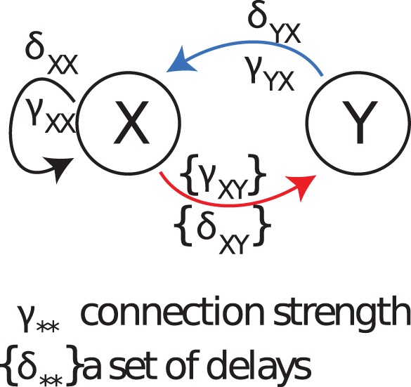
Transfer entropy () values and significance as a function of the assumed delay for two unidirectionally coupled autoregressive systems. For visualization purposes all values were normalized by the maximal value of the TE between the two systems, i.e. . Red and blue color indicate normalized transfer entropy values and significances for interactions and , respectively. The nominal interaction delay used for the generation of the data was 20 sampling units from the process to . Asterisks indicate those values of for which the p-value 0.05 once corrected for multiple comparisons. Missing points for are because the analyses for these ’s failed to pass the shift test (a conservative test in TRENTOOL to detect potential instantaneous cross-talk or shared noise between the two time series, see [42]).

Figure 6. Test case (III).

Transfer entropy () values and significance as a function of the assumed delay for two unidirectionally coupled autoregressive systems with multiple delays. The simulated delays were 15, 20, 25, 30 and 35 sampling points. The rest of the parameters and criteria used are the same as those in Figure 5.

Figure 7. Test case (IV).

Transfer entropy () values and significance as a function of the assumed delay for two unidirectionally coupled autoregressive systems with multiple delays. The simulated delays were 18, 19, 20, 21 and 22 sampling points. The rest of the parameters and criteria used are the same as those in Figure 5.

Figure 8. Test case (V).

Transfer entropy () values and significance as a function of the assumed delay for two bidirectionally coupled, chaotic Lorenz systems. The simulated delays were and , and the coupling constants were . The delays were recovered as and . For more parameters see table 2.

Figure 9. Test case (V).

Crosscorrelation function for the two quadratically coupled chaotic Lorenz systems from figure 8.

Figure 10. Test case (V) analyzed with the old estimator.

Transfer entropy () values and significance estimated by the old estimator from references , , , as a function of the assumed delay for two bidirectionally coupled, chaotic Lorenz systems. The simulated delays were and . These delays were recovered erroneously as and . For more parameters see table 2.

Figure 11. Test case (VI) - self-feedback analysis.

Transfer entropy () values between past and present of one of two Lorenz systems () and significances as a function of the assumed delay . The analyzed chaotic Lorenz system was subject to a feedback loop with delay , and an outgoing interaction with delay , but no incoming interaction. The recovered delay for the self feedback was , with a sidepeak at around two times this value. For the interaction analysis see figure 12. For more parameters see table 2.

Figure 12. Test case (VI).

Transfer entropy () values and significance as a function of the assumed delay for a unidirectionally coupled chaotic Lorenz systems. The first Lorenz is subject to a feedback loop () and unidirectionally couples to a second Lorenz with a interaction delay of samples. Recovered delays were (see figure 11), and . Sidepeaks were observed for close to . Spurious interactions were observed in the reversed direction at , as it is expect for a system with self feedback . Considering the positive test for self-feeback (figure 11) and the recovery of the self-feedback delay, the true system connectivity can be derived by combining the analysis of self-feedback and interaction delays.

Figure 13. Test case (VII) - self-feedback analysis.

Transfer entropy () values between past and present of one of two Lorenz systems () and their significances as a function of the assumed delay for a single chaotic Lorenz system subject to a feedback loop with delay , and an outgoing interaction with delay . The recovered delay for the self feedback was , with a sidepeak at two times this value. For the interaction analysis see figure 14. For more parameters see table 2.

Figure 14. Test case (VII).

Transfer entropy () values and significance as a function of the assumed delay for a unidirectionally coupled chaotic Lorenz systems. The first Lorenz is subject to a feedback loop () and unidirectionally couples to a second Lorenz with a interaction delay of samples. Recovered delays were (see figure 13), and . Sidepeaks were observed for close to . Spurious interactions were observed in the reversed direction at , as it is expect for a system with self feedback . Considering the positive test for self-feeback (figure 13) and the recovery of the self-feedback delay, the true system connectivity can be derived by combining the analysis of self-feedback and interaction delays.

Figure 15. Test case VIII.

Transfer entropy () values and significance as a function of the assumed delay for three unidirectionally coupled chaotic Lorenz systems. The First Lorenz couples with the second Lorenz with an interaction delay of samples, the second Lorenz is unidirectionally coupled with the third Lorenz at a delay of samples and the third Lorenz is unidirectionally coupled with the first Lorenz at an interaction delay of samples. The reconstruction of the simulated delays were: (A) self feedback, , this value may be due to insufficient embedding, (B) , (C) , and (D).

Figure 16. Test case IX.

Transfer entropy () values and significance as a function of the assumed delay for two bidirectionally coupled, chaotic Lorenz systems. The simulated delays were and . Observation noise with different amplitude was added to the simulated time series of the processes. The delays were recovered as (A) and for (blue), and (B) for (red) and and for (green).

Figure 17. Interaction delay reconstruction in the turtle brain.

(A) Electroretinogram (green), and LFP recordings (blue), light pulses are marked by yellow boxes. (B) Schematic depiction of stimulation and recording, including the investigated interactions and the identified delays.

References

-
- Pearl J (2000) Causality: models, reasoning, and inference. Cambridge University Press.
- Ay N, Polani D (2008) Information ows in causal networks. Adv Complex Syst 11: 17.
Publication types
MeSH terms
LinkOut - more resources
Full Text Sources
Other Literature Sources