Teaching basic principles of neuroscience with computer simulations

Abstract

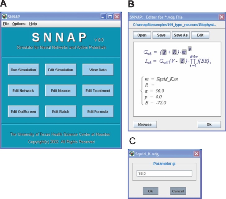
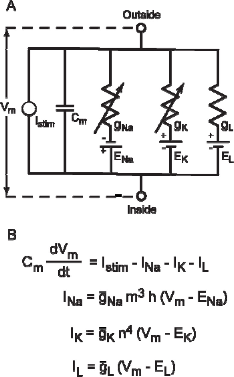
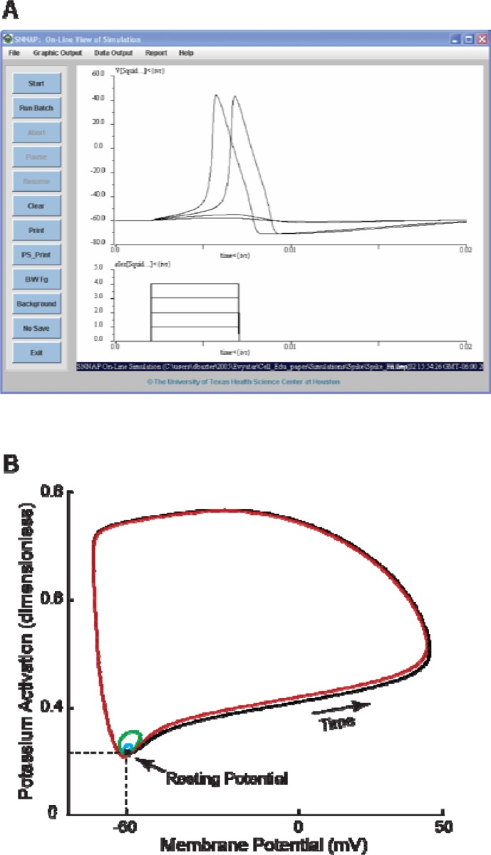
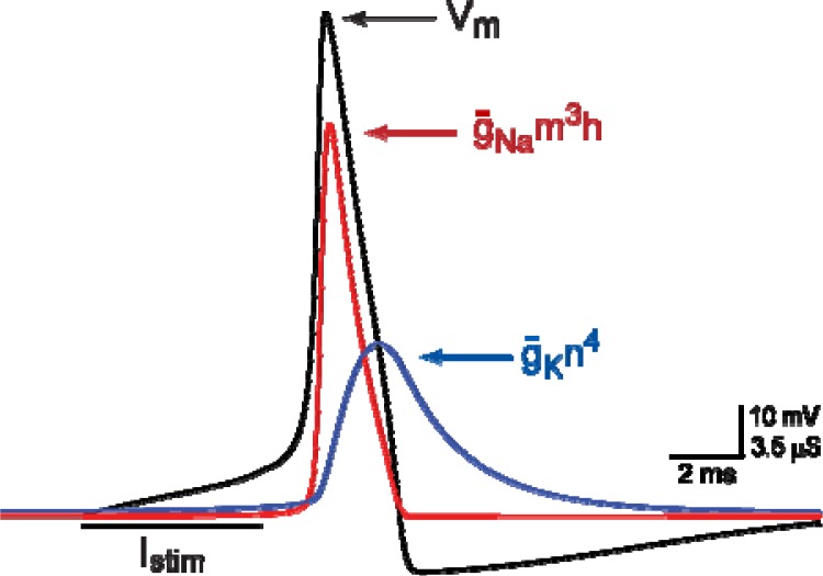
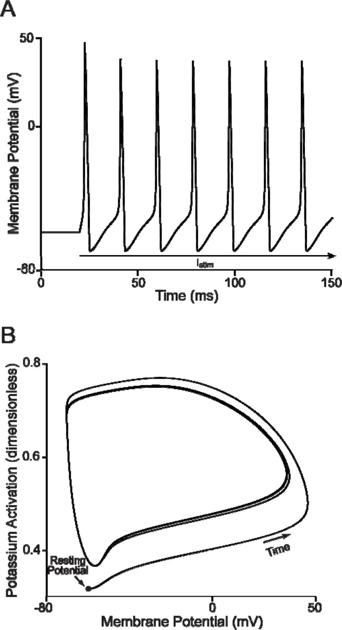
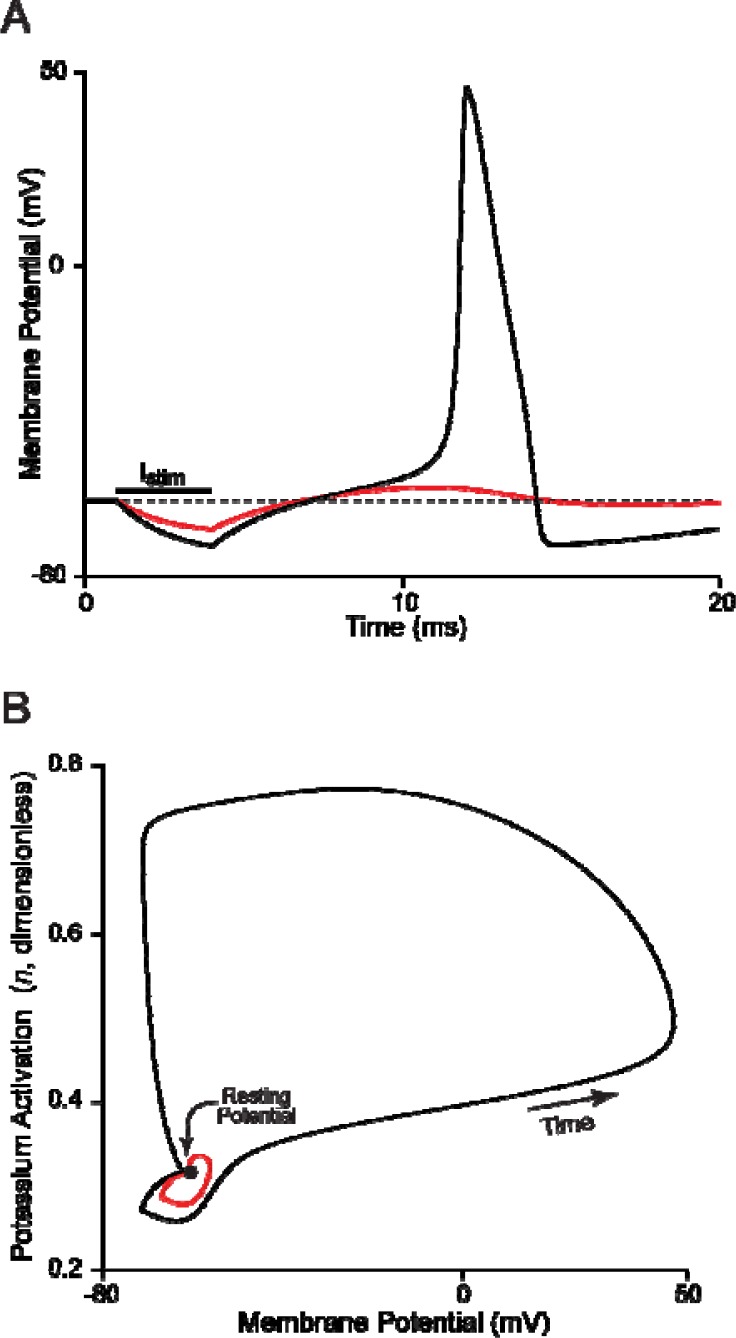
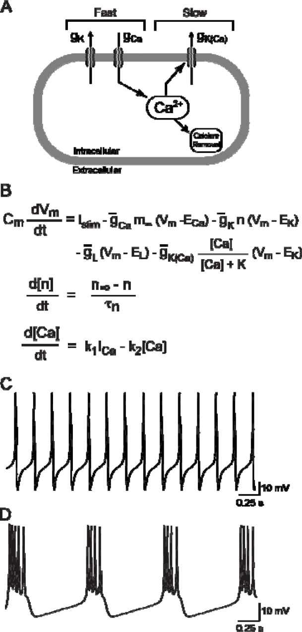
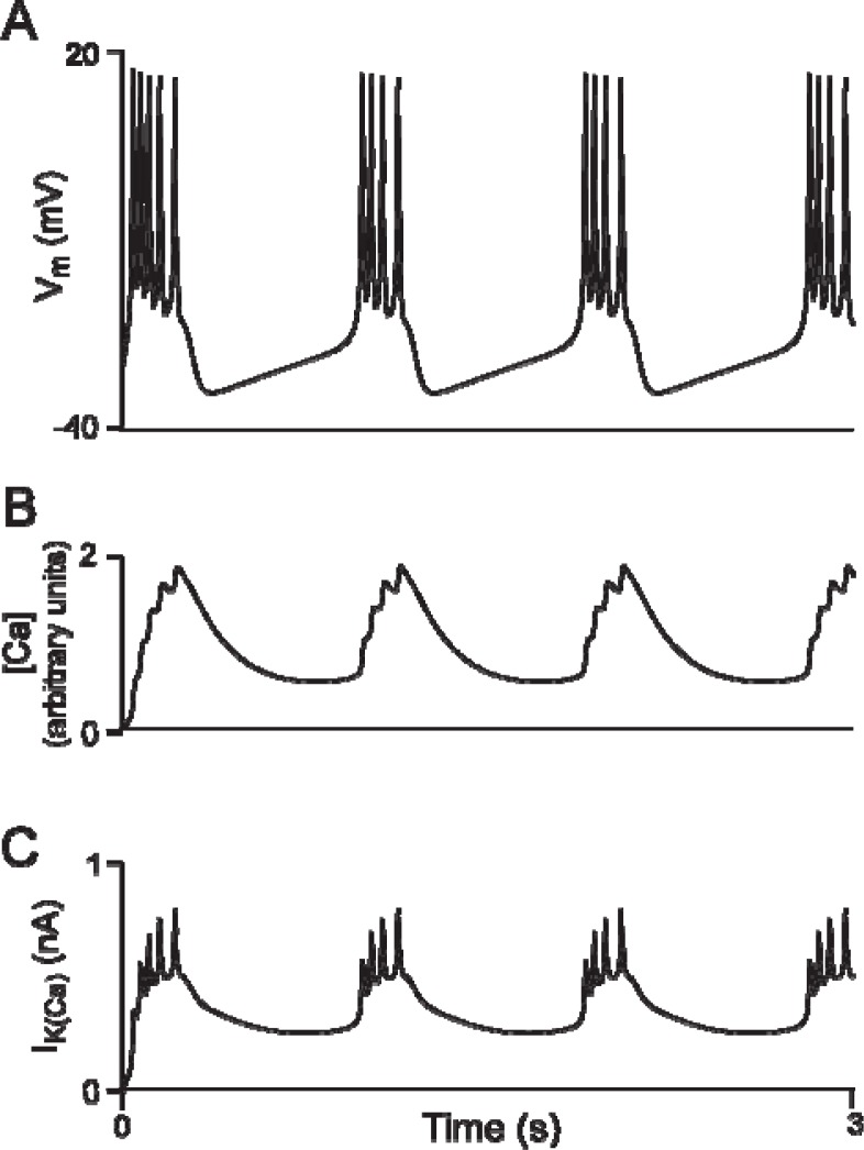
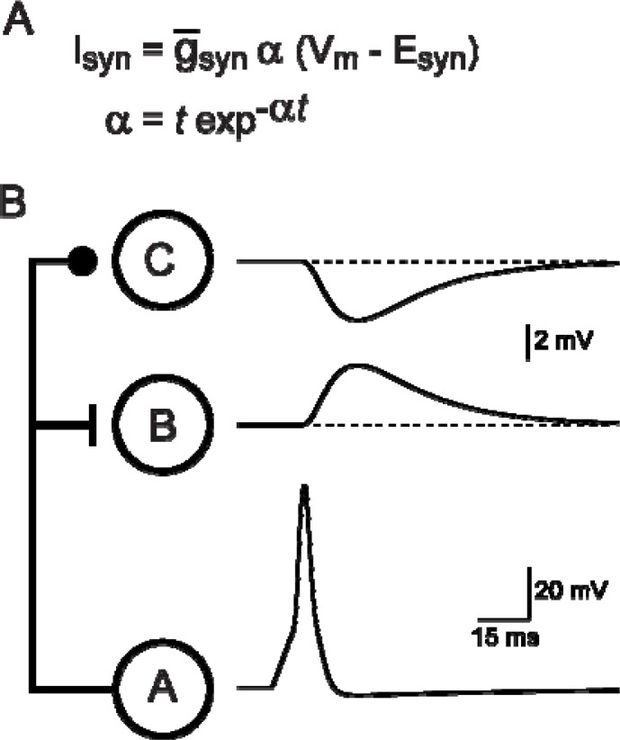
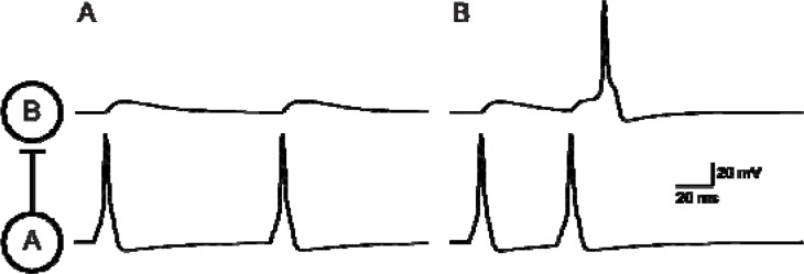
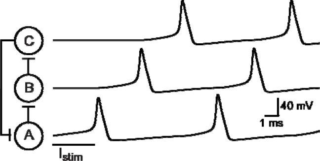
It is generally believed that students learn best through activities that require their direct participation. By using simulations as a tool for learning neuroscience, students are directly engaged in the activity and obtain immediate feedback and reinforcement. This paper describes a series of biophysical models and computer simulations that can be used by educators and students to explore a variety of basic principles in neuroscience. The paper also suggests 'virtual laboratory' exercises that students may conduct to further examine biophysical processes underlying neural function. First, the Hodgkin and Huxley (HH) model is presented. The HH model is used to illustrate the action potential, threshold phenomena, and nonlinear dynamical properties of neurons (e.g., oscillations, postinhibitory rebound excitation). Second, the Morris-Lecar (ML) model is presented. The ML model is used to develop a model of a bursting neuron and to illustrate modulation of neuronal activity by intracellular ions. Lastly, principles of synaptic transmission are presented in small neural networks, which illustrate oscillatory behavior, excitatory and inhibitory postsynaptic potentials, and temporal summation.

Keywords: Hodgkin-Huxley; SNNAP; graduate; modeling; neural networks; neurons; synapses; undergraduate.

Figure 1.

User-friendly interface for building models and running simulations. In SNNAP, all aspects of developing a model and running simulations can be controlled via a graphical-user interface (GUI; see also Fig. 3A). A: The simplest way to run SNNAP is to double click on the snnap.jar file. The first window to appear is the main control window. Other features of the neurosimulator are selected by clicking on the appropriate button. B: For example, clicking on the Edit Formula button invokes a file manager (not shown) and allows the user to select the file that contains the specific formula to be edited (in this case the hhK.vdg file). Once selected, the formula is displayed in the formula editor. The parameters in the formula are displayed with a shaded background. The current values for the parameters are listed in the lower portion of the display. C: To change the value of a parameter, click on the parameter. A dialog box appears and the user enters the new value. The SNNAP Tutorial Manual provides detailed instructions for operating SNNAP. The tutorial is available for download at the SNNAP website.

Figure 2.

Equivalent electric circuit for HH model. A: Hodgkin and Huxley pioneered the concept of modeling the electrical properties of nerve cells as electrical circuits. The variable resistors represent the voltage- and/or time-dependent conductances. (Note, conductances can also be regulated by intracellular ions or second messengers, see Fig. 7.) The HH model has three ionic conductances: sodium (g_Na), potassium(g_K) and leak (g_L). The batteries represent the driving force for a given ionic current. C_M represents the membrane capacitance. I_stim represents an extrinsic stimulus current that is applied by the experimenter. B: A few of the equations in the HH model. The ordinary differential equation (ODE) that describes the membrane potential (V_m) of the model contains the ensemble of ionic currents that are present. The HH model is relatively simple and contains only three ionic currents. Other models may be more complex and contain many additional ionic currents in the ODE for the membrane potential (e.g. see Butera et al., 1995; Av-Ron and Vidal, 1999). The ionic currents are defined by a maximal conductance (g̅), a driving force (V_m – E_ion), and in some cases activation (m, n) and/or inactivation (h) functions. These equations illustrate many of the parameters that students may wish to vary. For example, values of g̅ can be varied to simulate different densities of channels or the actions of drugs that block conductances. Similarly, values of E_ion can be changed to simulate changes in the extracellular concentrations of ions (see Av-Ron et al., 1991).

Figure 3.

Action potentials and threshold phenomena. A: Screen shot of the SNNAP simulation window. The upper trace illustrates the membrane potential of the HH model. The lower trace illustrates the extrinsic stimulus currents that were injected into the cell during the simulations. With each simulation, the magnitude of the stimulus is systematically increased in 1 nA increments. The first two stimuli are subthreshold, but the final two stimuli are suprathreshold and elicit action potentials. This figure also illustrates several features of the SNNAP simulation window. To run a simulation, first select File, which invokes a drop-down list of options. From this list select the option Load Simulation, which invokes a file manager (not shown). The file manager is used to select the desired simulation (*.smu file). Once the simulation has been loaded, pressing the Start button begins the numerical integration of the model and the display of the results. See the SNNAP Tutorial Manual for more details. B: Phase-plane representation of the threshold phenomena. The data in Panel A are plotted as time series (i.e., V_m versus time). Alternatively, the data can be plotted on a phase plane (i.e., potassium activation, n, versus membrane potential, V_m). Although time is not explicitly included in the phase plane, the temporal evolution of the variables proceeds in a counter-clockwise direction (arrow). The resting membrane potential is represented by a stable fixed point (filled circle at the intersection of the two dashed lines). The stimuli displace the system from the fixed point. If the perturbations are small, the system returns to the fixed point (small blue and green loops). However, for sufficiently large perturbations, the system is forced beyond a threshold and the trajectory travels in a wide loop before returning to the stable fixed point (red and black loops). The system is said to be excitable because it always returns to the globally stable fixed point of the resting potential. For more details concerning the application of phase plane analyses to computation models of neural function see Baxter et al. (2004), Canavier et al. (2005), or Rinzel and Ermentrout (1998).

Figure 4.

Conductance changes underlying an action potential. The membrane potential (V_m) is illustrated by the black trace. The sodium conductance (g̅_Nam³h) is illustrated by the red trace, and potassium conductance (g̅_K n⁴) is represented by the blue trace (see Fig. 2B). In response to the depolarizing stimulus (I_stim), the sodium conductance increases, which depolarizes the membrane potential and underlies the rising phase of the spike. The potassium conductance increases more slowly and underlies the falling phase of the action potential.

Figure 5.

Induced oscillatory behavior. A: The HH model oscillates if a constant, suprathreshold stimulus is applied. Note that the first spike has a larger amplitude due to the model starting from the resting potential; whereas, subsequent spikes arise from an afterhyperpolarization. B: Limit cycle. The simulation in Panel A is replotted on the V_m-n phase plane. After an initial transient, the trajectory of each action potential superimpose, which indicates the presence of a limit cycle. The constant stimulus destabilizes the fix point and the system exhibits limit cycle dynamics.

Figure 6.

Postinhibitory rebound excitation. A: Response of the HH model to hyperpolarizing current (I_stim) injected into the cell. Weak hyperpolarizing current (red curve), strong hyperpolarizing current (black curve). Following these inhibitory inputs, the membrane potential returns toward rest. The recovery of the membrane potential, however, overshoots the original resting membrane and depolarizes the cell. With sufficiently large hyperpolarization, the rebound potential surpasses the threshold and an action potential is elicited. B: The simulations illustrated in Panel A are replotted in the V_m-n phase plane. The hyperpolarizations are represented by hyperpolarizing displacements of the membrane potential and decreases in the value of potassium activation. Following the hyperpolarizing stimulus, the trajectory moves back toward the resting potential, which is represented by a fixed point (filled circle). However, the trajectory that follows the larger hyperpolarization crosses a threshold (also referred to as a separatrix) and an action potential is generated.

Figure 7.

Morris-Lecar (ML) model. A: Schematic representing elements of the ML model. Similar to the HH model, the ML model has two fast ionic conductances (g_Ca, g_K) that underlie spike activity. However, in the ML model the inward current is calcium rather than sodium. To implement bursting, the ML model was extended to include an intracellular pool of calcium and a second, calcium-dependent potassium conductance (g_K(Ca)). The kinetics of the calcium pool are relatively slow and determined the activation kinetics of the calcium-dependent potassium conductance. B: The ordinary differential equations (ODEs) that define the ML model. The ODEs for membrane potential V_m and potassium activation n, are similar to that for the HH model, however, a new term is added to describe the calcium-activated potassium current I_K(Ca). The activation of g_K(Ca) is determined by a function of calcium concentration ([Ca]/([Ca]+K)), and [Ca] is defined by an ODE in which the calcium current (k₁I_Ca) contributes calcium to the ion pool and buffering (−k₂[Ca]) removes calcium from the ion pool. C: If the intracellular pool of calcium and the calcium-activated potassium conductance are not included, the ML model exhibits oscillatory behavior in response to a sustained, suprathreshold stimulus. D: With the intracellular pool of calcium and the calcium-activated potassium conductance in place, the ML model exhibits bursting behavior in response to a sustained suprathreshold stimulus. The burst of spikes are superimposed on a depolarizing wave, which is mediated by calcium current. The interburst period of inactivity is mediated by the calcium-dependent potassium current (see Fig. 8).

Figure 8.

Mechanisms underlying bursting behavior of the ML model. A: Membrane potential during bursting. B: During the burst of action potentials (Panel A), the intracellular levels of calcium slowly increase. C: As the levels of calcium increase (Panel B), the calcium-dependent potassium conductance increases. Eventually, the calcium-dependent potassium current is sufficiently large to halt spiking and a period of inactivity follows (Panel A). During the quiescent period, the level of calcium falls (Panel B) and the activation of the potassium current decreases (Panel C). This allows the membrane potential to slowly depolarize back toward threshold and another burst of spikes is initiated. Therefore, bursting originates from the interactions between a fast (calcium/potassium) spiking process and a slow (intracellular calcium/calcium-activated potassium) inhibitory process (see Fig. 7A).

Figure 9.

Excitatory and inhibitory postsynaptic potentials (EPSPs and IPSPs). A: Similar to ionic currents (see Fig. 2B), synaptic currents are defined by a maximum conductance (g̅_syn), a time-dependent activation function (α) and a driving force (V_m – E_syn). An expression that is commonly used to define the time-dependent activation function is referred to as an alpha (α) function, which resembles the time course of empirically observed synaptic currents. SNNAP offers several additional functions for defining synaptic activation, including functions that incorporated both time- and voltage-dependency. B: In this simple neural network, a single presynaptic cell (A) makes synaptic connections with two postsynaptic cells (B and C). The connection from A to B is excitatory, whereas the connection from A to C is inhibitory. The only difference between the two synaptic models is the value for E_syn. For excitatory synapses, E_syn is more depolarized than the resting membrane potential; whereas for inhibitory synapses, E_syn is more hyperpolarized than the resting potential.

Figure 10.

Temporal summation. A network of two neurons with an excitatory synapse from cell A to cell B. A: Two presynaptic action potentials are elicited with an interspike interval of 100 ms. The individual EPSPs are subthreshold for eliciting a postsynaptic spike. B: If the interspike interval is reduced to 50 ms, the EPSPs summate and elicit a postsynaptic spike. The temporal summation of the two EPSPs produces a suprathreshold depolarization in the postsynaptic cell and a spike is elicited.

Figure 11.

Three cell neural network with recurrent excitation. Three HH models connected in a ring-like architecture. All synaptic connections are excitatory. An initial, brief stimulus to cell A (I_stim.) elicits a single action potential, which in turn, produces suprathreshold EPSP in cell B, which in turn, produces a suprathreshold EPSP in cell C. Cell C excites cell A and the cycle repeats itself indefinitely.

References

1. Abbott L, Marder E. Modeling small networks. In: Koch C, Segev I, editors. Methods in neuronal modeling: from ions to networks. 2nd edition. Cambridge, MA: The MIT Press; 1998. pp. 363–410.
1. Abraham RH, Shaw CD. Dynamics: the geometry of behavior. 2nd edition. Redwood City, CA: Addison-Wesley; 1992.
1. Av-Ron E, Parnas H, Segel LA. A minimal biophysical model for an excitable and oscillatory neuron. Biol Cybern. 1991;65:487–500. - PubMed
1. Av-Ron E, Vidal PP. Intrinsic membrane properties and dynamics of medial vestibular neurons: a simulation. Biol Cybern. 1999;80:383–392. - PubMed
1. Av-Ron E, Cai Y, Byrne JH, Baxter DA. Soc. Neurosci. Abstr. Washington, DC: Society for Neuroscience; 2004. An interactive and educational tutorial for version 8 of SNNAP (Simulator for Neural Networks and Action Potentials) Program No. 27.13, 2004 Abstract Viewer/Itinerary Planner. Online: sfn.scholarone.com/itin2004/
LinkOut - more resources