Teaching basic neurophysiology using intact earthworms

Abstract

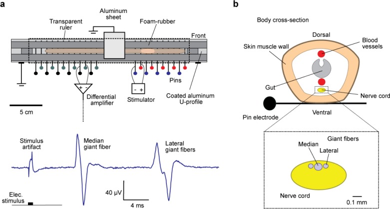
Introductory neurobiology courses face the problem that practical exercises often require expensive equipment, dissections, and a favorable student-instructor ratio. Furthermore, the duration of an experiment might exceed available time or the level of required expertise is too high to successfully complete the experiment. As a result, neurobiological experiments are commonly replaced by models and simulations, or provide only very basic experiments, such as the frog sciatic nerve preparation, which are often time consuming and tedious. Action potential recordings in giant fibers of intact earthworms (Lumbricus terrestris) circumvent many of these problems and result in a nearly 100% success rate. Originally, these experiments were introduced as classroom exercises by Charles Drewes in 1978 using awake, moving earthworms. In 1990, Hans-Georg Heinzel described further experiments using anesthetized earthworms. In this article, we focus on the application of these experiments as teaching tools for basic neurobiology courses. We describe and extend selected experiments, focusing on specific neurobiological principles with experimental protocols optimized for classroom application. Furthermore, we discuss our experience using these experiments in animal physiology and various neurobiology courses at the University of Bonn.

Keywords: action potentials; conduction velocity; earthworms; extracellular recordings; facilitation of conduction velocity; flight reflexes; giant fibers; giant motorneuron; refractory period; spatial size of action potentials; synaptic depression and facilitation; threshold.

Figure 1

Experimental setup. (a) The setup for recording giant fiber activity in intact earthworms is illustrated. Basically, the intact earthworm is placed in a cage that maximally restricts locomotion. An array of electrodes comes into contact with the outer ventral side of the worm. These electrodes are plain stainless steel household pins and serve as recording, as well as stimulation electrodes. A transparent ruler, clamped above, completes the cage. This ruler can be shifted to allow mechanical stimulation of the worm. The trace shows an extracellular recording of the median and lateral giant fiber responses following an electrical stimulus (classroom data). (b) A body cross-section through the earthworm is shown. The nerve is located ventrally, close to the pin electrodes beneath the worm. The inset illustrates the dorsal location of the three giant fibers within the ventral nerve cord.

Figure 2

Components of the flight reflex, mediated by the MGF pathway. Mechanical stimulation of the worm front end leads to activity in skin sensory cells. This activates sensory interneurons that are connected to the median giant fiber. The MGF is connected to segmental giant motorneurons that elicit contraction of longitudinal muscles in the body wall. A positive feedback loop, via a single interneuron, can enhance the flight reflex by eliciting a second, or even several more, action potentials of the MGF.

Figure 3

Changes in membrane excitability following an action potential. (a) Example of action potentials elicited by double pulses. The measurement was performed using method 1, varying intervals but constant width and strength (0.5 ms, 2.8 mA). At intervals larger than 20ms, the amplitude of the second AP (green dots) is the same than the first AP. At some point, the second AP becomes smaller (relative refractory period, light green bar), until it completely vanishes (absolute refractory period, dark green bar). Using method 2 (measuring the threshold for eliciting a second AP), we get somewhat different values for the refractory periods (dark red and light red bar). (b) Comparison of the conduction velocities of the first and second AP of two different earthworms. If the second AP is elicited 5–8 ms after the first AP, it has a higher conduction velocity. However, close to the absolute refractory period, it has a lower velocity.

Figure 4

Spatial dimensions of action potentials. (a) Experimental setup. (b) The conduction of action potentials. An electrical stimulus leads to the generation of an action potential by depolarizing the membrane; in this case the median giant fiber. This depolarization leads to a negative potential wave caused by current loops. As the negative potential wave is conducted along the fiber, the amplitude of the recording depends on the difference between the two electrodes (+/-). This difference is dependent on electrode distance, i.e., if the negative potential wave fits in between the electrodes (setting II), there is no potential difference measured for a short period of time and this results in a plateau showing up in the recordings. (c) Examples of classroom traces for electrodes placed at distances of 1 and 2 cm (I/II).

Figure 5

Spatial dimensions of the MGF and LGF responses. An example of four recordings of the MGF and LGF with different electrode distances (2, 5, 10 and 15 mm) is shown. The plateau of the MGF is given at a distance of 15 mm and for the LGF there already is a plateau at a distance of 10 mm (black arrows).

Figure 6

Methods to calculate the conduction velocity. If possible, a double recording is used to calculate the conduction velocity (b). Here, the time between the two recording electrodes (-/-) and the distance between these is used for the calculations. If a double recording is not an option, the distance between the stimulus and the recording electrodes as well as the latency can be used to estimate the conduction velocity (a).

Figure 7

Strength-duration curves. (a) Representative student measurements of the MGF strength-duration curve. In this example, we used 24 different stimulus durations and amplitudes up to 2.8 mA. The minimal electric current (rheobase) of the MGF is at 0.19 mA and the chronaxy is at 129 μs. (b) The strength-duration curve of the LGF shows a rheobase of 0.3 mA and a chronaxy of 177 μs.

Figure 8

Synaptic depression of giant motorneurons. (a) Experimental setup. (b) In weakly anesthetized worms, the MGF response is followed by the summation of the action potentials of six segmental giant motorneurons. By overdrawing all responses to the 30 Hz stimuli, it becomes clear that the motorneuron response does not diminish continuously but in steps, according to failure of one synapse after the other.

Figure 9

Mechanical stimulation of the worm front end, activating the MGF pathway. (a) Experimental setup. (b) Two traces of recordings following a mechanical stimulus are shown. In the upper trace, the stimulus leads to a response of the MGF, followed by motorneuron responses. The lower trace shows the action of the positive feedback loop. The first MGF response is followed by the motorneurons and a few muscle potentials. In addition, a second MGF response can be observed after a delay (positive feedback loop), again followed by motorneuron responses and now much stronger muscle potentials (facilitation).

Figure 10

Mechanical stimulation of the worm hind end, activating the LGF pathway. (a) Experimental setup. (b) Classroom measurements following three stimuli with different strengths are shown. After weak stimuli, usually one AP with a high latency is recorded. The number of APs increases with stimulus strength, while their latency decreases. After strong stimuli, muscle potentials are typically seen, along with strong twitches of the worm.

Figure 11

Conduction velocities of LGF responses. With a double recording, students can measure the decrease in conduction delay in subsequent APs. In this example, students measured the conduction velocities of the first three LGF responses. In this measurement, the intervals between the two recordings were 6.8 ms (first AP), 5.9 ms (second AP) and 5.5 ms (third AP) and the distance of the two recording sites was 70 mm. The calculated conduction velocities increase from 10.3 m/s for the first AP, 11.9 m/s for the second AP to 12.7 m/s for the third AP.

Figure 12

Temperature dependency of the conduction velocity. A classroom calculation of the conduction velocity of the MGF (red line) and LGF (blue line) is shown. In this case the experiment starts at room temperature and over time, the worm is cooled down to 2 °C.

References

1. Ballo AW, Bucher D. Complex intrinsic membrane properties and dopamine shape spiking activity in a motor axon. J Neurosci. 2009;29:5062–5074. - PMC - PubMed
1. Bear MF, Connors BW, Paradiso MA. Neuroscience, exploring the brain. 3rd ed. Baltimore, MD: Lippincott Williams and Wilkins; 2007.
1. Bullock TH. Functional organization of the giant fibre system of Lumbricus. J Neurophysiol. 1945;8:54–71.
1. Bullock TH. Facilitation of conduction rate in nerve fibers. J Physiol. 1951;114:89–97. - PMC - PubMed
1. Bullock TH, Horridge GA. Structure and function in the nervous systems of invertebrates. San Francisco, CA: Freeman and Company; 1965.
LinkOut - more resources