Characterizing the ear canal acoustic impedance and reflectance by pole-zero fitting

Abstract

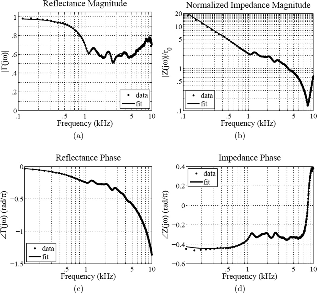
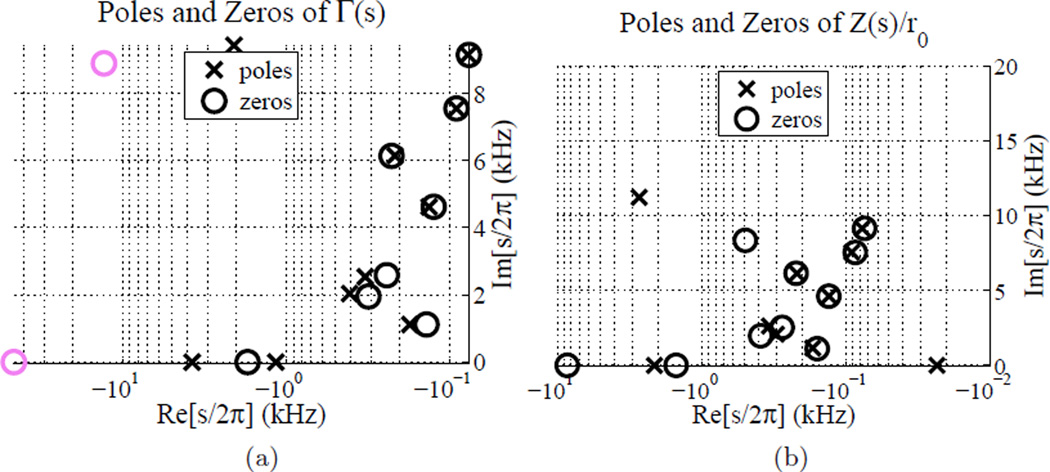
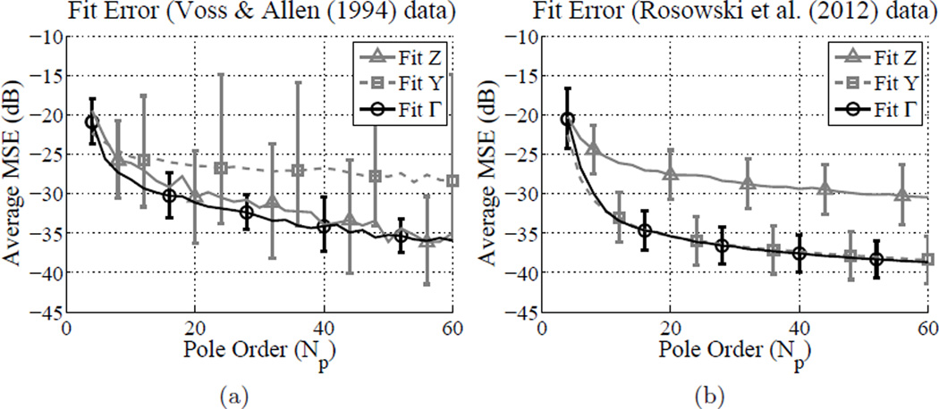
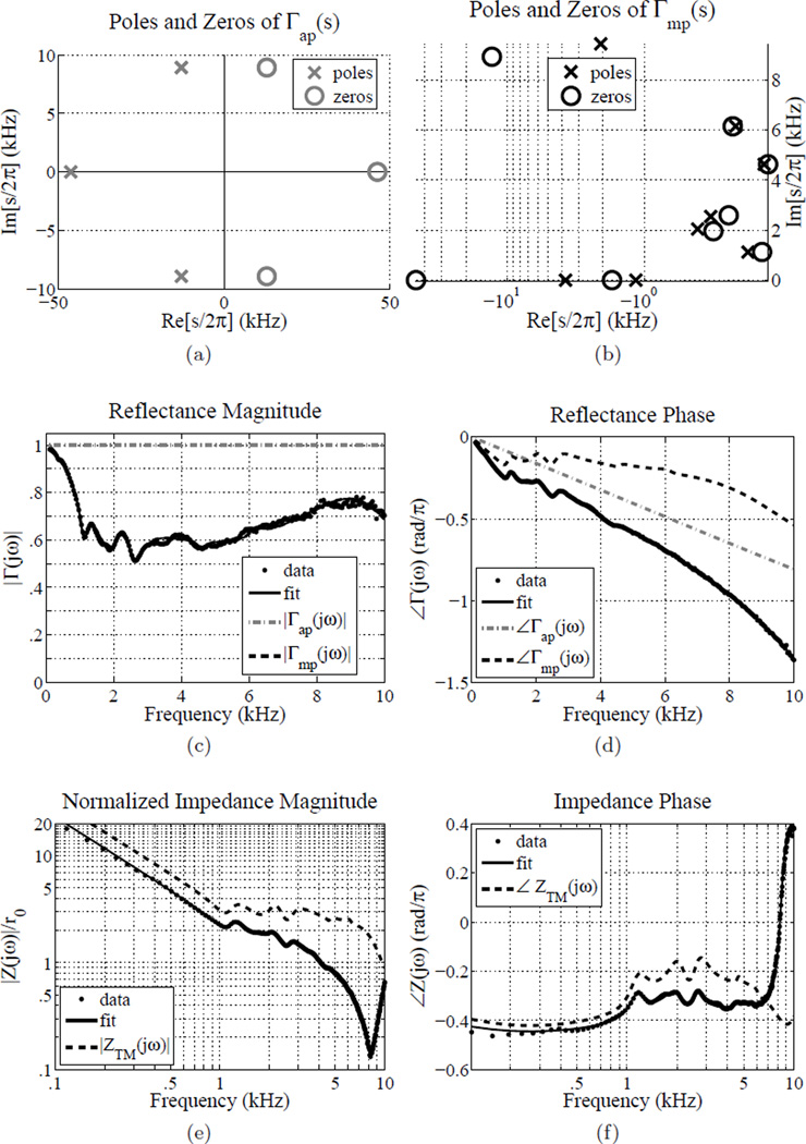
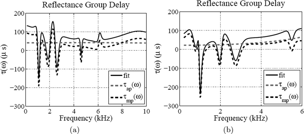
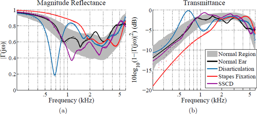
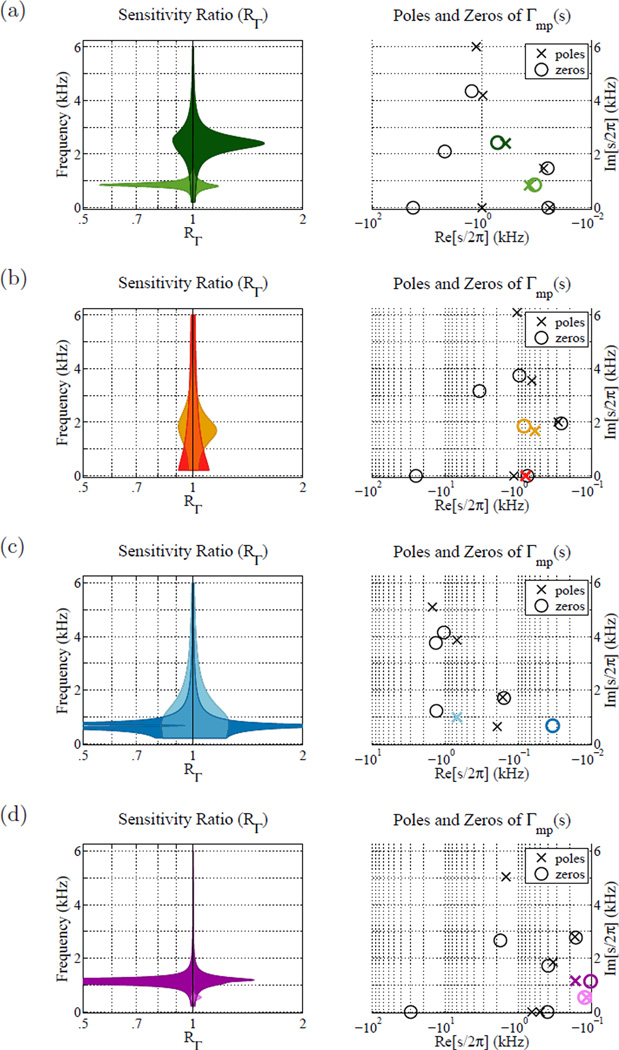
This study characterizes middle ear complex acoustic reflectance (CAR) and impedance by fitting poles and zeros to real-ear measurements. The goal of this work is to establish a quantitative connection between pole-zero locations and the underlying physical properties of CAR data. Most previous studies have analyzed CAR magnitude; while the magnitude accounts for reflected power, it does not encode latency information. Thus, an analysis that studies the real and imaginary parts of the data together, being more general, should be more powerful. Pole-zero fitting of CAR data is examined using data compiled from various studies, dating back to Voss and Allen (1994). Recent CAR measurements were taken using the Mimosa Acoustics HearID system, which makes complex acoustic impedance and reflectance measurements in the ear canal over a 0.2-6.0 [kHz] frequency range. Pole-zero fits to measurements over this range are achieved with an average RMS relative error of less than 3% with 12 poles. Factoring the reflectance fit into its all-pass and minimum-phase components estimates the effect of the residual ear canal, allowing for comparison of the eardrum impedance and admittance across measurements. It was found that individual CAR magnitude variations for normal middle ears in the 1-4 [kHz] range often give rise to closely-placed pole-zero pairs, and that the locations of the poles and zeros in the s-plane may systematically differ between normal and pathological middle ears. This study establishes a methodology for examining the physical and mathematical properties of CAR using a concise parametric model. Pole-zero modeling accurately parameterizes CAR data, providing a foundation for detection and identification of middle ear pathologies. This article is part of a special issue entitled "MEMRO 2012".

Figure 1

Voss and Allen (1994) subject #7; example data and fit for a normal ear. (a) Reflectance magnitude, (b) impedance magnitude, (c) reflectance phase, (d) impedance phase. The fit was performed over 0.1 to 10 kHz, yielding 18 poles and 18 zeros with an RMS relative error of 2.5% (MSE = −31.9 dB).

Figure 2

Voss and Allen (1994) subject #7; example pole-zero fit for a normal ear. (a) Poles and zeros of Γ(s), (b) poles and zeros of Z(s). The fit was performed over 0.1 to 10 kHz, yielding 18 poles and 18 zeros with an RMS relative error of 2.5% (MSE = −31.9 dB). Pink poles and zeros are actually located in the positive real s-plane, but have been inverted over the jω axis so that pole-zero locations may be more easily viewed using a log ℜ[s] axis.

Figure 3

Fit error evaluation across the Z, Y and Γdomains for different data sets (18 iterations). Lines show the average MSE (dB) for each domain, with error bars indicating one standard deviation. (a) 14 measurements of normal ears (Voss and Allen, 1994) fit over the 0.1 to 10 kHz range, (b) 112 measurements of normal ears (Rosowski et al., 2012) fit over the 0.2 to 6 kHz range.

Figure 4

Voss and Allen (1994) subject #7; example of a factored reflectance fit. (a) Poles and zeros of Γ_ap(s), (b) poles and zeros of Γ_mp(s), (c) reflectance magnitude, (d) reflectance phase, (e) impedance magnitude, (f) impedance phase. Note that Γ_mp(s) has no poles or zeros in the positive real s-plane, thus the fit is completely described by 4^th quadrant of the s-plane (shown in (b)) without any plotting tricks. All 4 quadrants of the s-plane are shown in plot (a) to allow the reader to view the symmetry of |Γ_ap(s)|. The fit was performed over 0.1 to 10 kHz, yielding N_p = 18 and N_z = 18 with an RMS relative error of 2.5% (MSE = −31.9 dB) as shown in Fig. ??; the pole-zero pairs at ℑ[s] ≈ 7.5 kHz and ℑ[s] ≈ 9 kHz were removed, yielding a MSE of −31.5 dB and N_p = 14 and N_z = 14.

Figure 5

Voss and Allen (1994) subject #7; example of a factored reflectance fit.(a) Poles and zeros of Γ_ap(s), (b) poles and zeros of Γ_mp(s), (c) reflectance magnitude, (d) reflectance phase, (e) impedance magnitude, (f) impedance phase. Note that Γ_mp(s) has no poles or zeros in the positive real s-plane, thus the fit is completely described by 4^th quadrant of the s-plane (shown in (b)) without any plotting tricks. All 4 quadrants of the s-plane are shown in plot (a) to allow the reader to view the symmetry of |Γ_ap(s)|. The fit was performed over 0.2 to 6 kHz, yielding N_p = 12 and N_z = 12 with a MSE = −35.8 dB.

Figure 6

Group delay of the fit Γ̂(s), and its factors Γ̂_mp(s) and Γ̂_ap(s). (a) Voss and Allen (1994) subject #7, (b) Voss et al. (2012) ear 12R (‘normal’ middle ear state).

Figure 7

A comparison of normal and pathological ears. (a) Power reflectance |Γ(jω)|², (b) transmittance level (dB). Grey region shows the normative region for the Rosowski et al. (2012) study of normal ears (±1 standard deviation). The black data points and line show the data and fit for normal ear 22L of Rosowski et al. (2012). The blue, red, and purple show the data and fit for stapes fixation ear 62L, disarticulation ear 28L, and SSCD ear 52L of Nakajima et al. (2012).

Figure 8

Sensitivity analysis of poles and zeros for the ears shown in Fig. 7. Each subplot shows the pole-zero plot Γ_mp(s) of the fit (left), and the corresponding sensitivity analysis of the highlighted poles (right). The sensitivity analysis represents a ratio of modified reflectance magnitude |Γ(jω)| to the original fit, given a slight variation in the location of the highlighted pole, zero, or pole-zero pair. Each sensitivity plot shows two different color-coded analyses. Notice that the frequency axes are aligned for each pair of plots. (a) Normal ear, (b) stapes fixation, (c) disarticulation, (d) SSCD.

References

-
- Allen J. Measurement of eardrum acoustic impedance. Peripheral Auditory Mechanisms. 1986;44
- Allen J, Jeng P, Levitt H. Evaluation of human middle ear function via an acoustic power assessment. Journal of Rehabilitation Research & Development. 2005;42:63–78. - PubMed
- Brune O. Synthesis of a finite two-terminal network whose driving-point impedance is a prescribed function of frequency. J of Math Phys. 1931;10:191–236.
- Farmer-Fedor B, Rabbitt R. Acoustic intensity, impedance and reflection coefficient in the human ear canal. The Journal of the Acoustical Society of America. 2002;112:600–620. - PubMed
- Feeney M, Grant I, Marryott L. Wideband energy reflectance measurements in adults with middle-ear disorders. Journal of Speech, Language, and Hearing Research. 2003;46:901–911. - PubMed
Publication types
MeSH terms
Grants and funding
LinkOut - more resources
Full Text Sources
Other Literature Sources