Functional characterization of the extraclassical receptive field in macaque V1: contrast, orientation, and temporal dynamics

Abstract

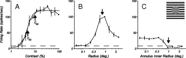
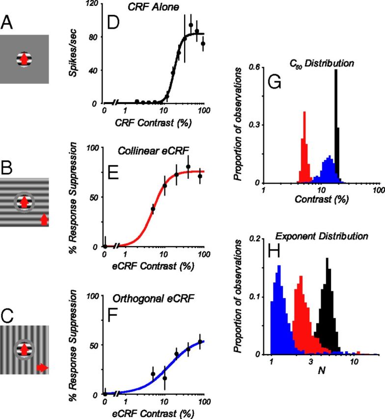
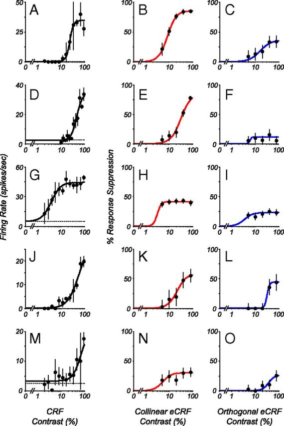
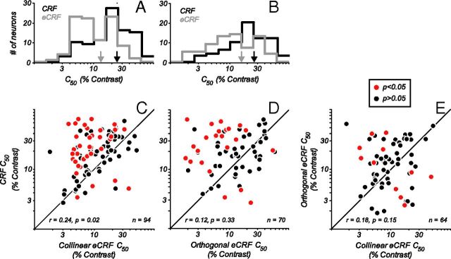
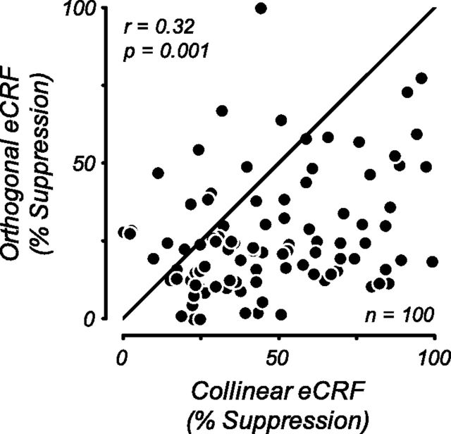
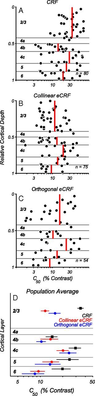
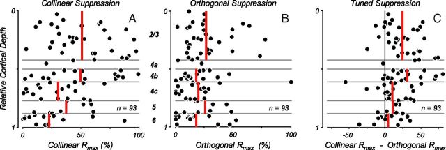
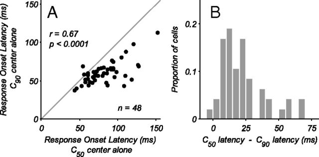
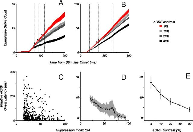
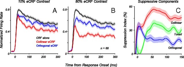
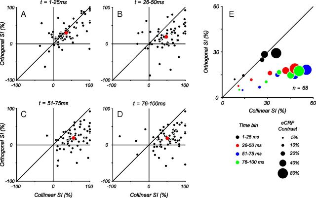
Neurons in primary visual cortex, V1, very often have extraclassical receptive fields (eCRFs). The eCRF is defined as the region of visual space where stimuli cannot elicit a spiking response but can modulate the response of a stimulus in the classical receptive field (CRF). We investigated the dependence of the eCRF on stimulus contrast and orientation in macaque V1 cells for which the laminar location was determined. The eCRF was more sensitive to contrast than the CRF across the whole population of V1 cells with the greatest contrast differential in layer 2/3. We confirmed that many V1 cells experience stronger suppression for collinear than orthogonal stimuli in the eCRF. Laminar analysis revealed that the predominant bias for collinear suppression was found in layers 2/3 and 4b. The laminar pattern of contrast and orientation dependence suggests that eCRF suppression may derive from different neural circuits in different layers, and may be comprised of two distinct components: orientation-tuned and untuned suppression. On average tuned suppression was delayed by ∼25 ms compared with the onset of untuned suppression. Therefore, response modulation by the eCRF develops dynamically and rapidly in time.

Figure 1.

Contrast response and size tuning for a complex cell. A, The response as a function of contrast for a grating of the optimal orientation, spatial and temporal frequency, and drift direction presented in a circular window that was the optimal size for the CRF. Closed circles and error bars indicate average firing rate (mean ± 1 SEM). The solid line is the best-fitting Naka–Rushton function. The arrows show the contrast eliciting 50 (C₅₀) and 90% (C₉₀) of the maximum response of the neuron, which were the contrasts used for subsequent contextual experiments. The dashed line indicates the spontaneous firing rate. B, The response as a function of the radius of the circular window containing an optimal grating as described in A. The arrow shows the smallest window radius eliciting the peak response of the neuron, which is the size of the central patch used in subsequent contextual experiments. C, A full-field optimal grating was presented that included a central gray circular region, where the radius of the central region varied from 0 to 4°, in 1/2 octave steps. The arrow shows the smallest radius of central blank gray region that elicited no response from the neuron. This size was used as the inner radius of stimuli presented to the eCRF and the outer radius of the gray annulus separating stimuli in the CRF from the eCRF (see the configuration in Fig. 2B,C).

Figure 2.

CRF and eCRF contrast response function comparison. A, Stimulus configuration for CRF alone, where a central patch of grating is optimized in orientation, spatiotemporal frequency, drift direction (red arrow), and size for the individual neuron. B, Stimulus configuration for CRF in the presence of a collinear eCRF, a central patch of grating as in A, simultaneously presented with a grating in the eCRF at the same spatiotemporal frequency and orientation. There was a small annular gray region that separated the center patch and the grating in the eCRF. The radius of the center patch was the optimal size for the CRF. The outer radius of the gray annulus was the size chosen from the expanding gray disk experiment where there was no response marked by the arrow in Figure 1C. C, Stimulus configuration for CRF in the presence of an eCRF stimulus oriented orthogonally to the central grating. For B and C, the gratings in the eCRF were presented at a range of contrasts, from 5 to 80%, in octave steps. D, The contrast response function for the CRF. E, Contrast-suppression function from the eCRF in response to collinear eCRF stimuli. F, Contrast-suppression function for orthogonal eCRF stimuli. D–F, The closed circles and error bars indicate mean ± 1 SD. Lines are best fits of the Naka–Rushton function to the data. For comparison of parameters between conditions, estimates of parameter distributions were achieved by repeated fitting to bootstrap samples of the data. G, Distributions of C₅₀. H, Distributions of exponent parameter, for CRF (black), collinear eCRF (red), and orthogonal eCRF (blue).

Figure 3.

Comparison of responses and suppression as a function of contrast in five neurons that show a range of CRF contrast-response functions and suppression strengths from the eCRF. Each row represents a different neuron. The first column (A, D, G, J, M) shows contrast responses from the CRF for the example cells (mean ± 1 SD). Second (B, E, H, K, N) and third (C, F, I, L, O) columns show the percentage suppression as a function of contrast from collinear- and orthogonal-oriented stimuli in the eCRF, respectively (mean ± 1 SD). Lines are best fits of the Naka–Rushton function to the data. Collinear suppression was generally stronger than orthogonal suppression, and C₅₀s from eCRF were generally equal to or lower than C₅₀s from CRF.

Figure 4.

Comparison of C₅₀ values from CRF with eCRF. A, Distribution of C₅₀ values from the Naka–Rushton function fitted to the contrast response of the CRF (black histogram) and contrast-dependent suppression from the collinear orientation in the eCRF (gray histogram). The arrows on the abscissa indicate the median values of each distribution. On average, eCRF C₅₀ values were lower than CRF C₅₀ values. B, Histogram of CRF C₅₀ and orthogonal eCRF C₅₀. C, Scatter plot of CRF and collinear eCRF C₅₀ values; points in red indicate a significant (p < 0.05) difference in the parameters. The majority of points lie above the unity line, indicating that within individual neurons eCRF C₅₀ values were significantly lower than CRF C₅₀ values. D, Scatter plot of CRF and orthogonal eCRF C₅₀ values. Again, the majority of points lie above the unity line. E, Scatter plot of C₅₀ values for both collinear and orthogonal eCRFs. For both orientations the eCRF C₅₀ distributions were centered around very low contrasts; however, there was no significant correlation between the two measures.

Figure 5.

Orientation-dependent eCRF suppression strength. Scatter plot of the maximum strength of suppression from collinear and orthogonal stimuli in the eCRF. Suppression strength was defined as the percentage suppression of CRF responses and was estimated as the R_max parameter from contrast response function fits to eCRF suppression. There was a significant correlation between the strength of eCRF suppression for collinear and orthogonal stimuli (r = 0.32, p = 0.001). Nearly all points lie below the unity line, indicating that there was consistently stronger suppression from the collinear eCRF stimulus.

Figure 6.

Contrast evoking half-maximal response (C₅₀) of CRF and eCRF across cortical layers. Measures of C₅₀ are plotted for excitation from the CRF and suppression from the eCRF in relation to the cortical depth of recordings. Red vertical lines indicate mean values within each layer. A, Laminar distribution of the C₅₀ parameter obtained from the best-fitting Naka–Rushton function to the CRF contrast responses for each neuron. On average, the contrast eliciting half-maximal excitation from the CRF was ∼20% for all layers and there was a trend for the lowest C₅₀s to occur in layers 4b and 6. B, Distribution of C₅₀ parameter values obtained for each neuron for eCRF suppression from collinear stimuli. Contrast sensitivity for suppression was high (C₅₀ ∼ 10% contrast) across all layers, even in layers 2 and 3 for which the CRF had a low-contrast sensitivity (A). C, The distribution of C₅₀ for suppression from orthogonal gratings in the eCRF. Even though orthogonal grating in the eCRF produced relatively weak suppression, the sensitivities were higher on average than those for CRF excitation. D, Summary plot of the average values for CRF (black squares) and eCRF C₅₀ (collinear, red circles; orthogonal, blue circles) across cortical layers (mean ±1 SD). eCRF C₅₀ values were lower than CRF values across all layers, with the largest differential in layers 2/3.

Figure 7.

Suppression indices across cortical layers. Measures of maximum suppression strength (R_max parameter of fit to response suppression as a function of contrast) are plotted as a function of cortical layer for conditions in which stimuli of either collinear or orthogonal orientation were presented within the eCRF, while the contrast in the CRF was the C₉₀ value for each neuron. R_max values of 0% indicate no modulation from eCRF stimulation and values near 100% indicate complete suppression of the neural response. Red vertical lines indicate mean values within each layer. A, The distribution of suppression strengths is shown for collinear stimuli in the eCRF. B, Distribution of suppression strengths for an orthogonal orientation in the eCRF. The suppression strength across layers with orthogonal stimuli was reduced compared with collinear orientation in the eCRF, yet there were still some neurons that showed strong suppression. C, The suppression strength of the orientation-tuned component, i.e., the differences in suppression between A and B, was greatest in layers 2/3 and 4b (24 ± 4% and 31 ± 7%, respectively) and much weaker in layers 5 (11 ± 4%) and 6 (5 ± 5%, mean ± SEM).

Figure 8.

Change in CRF response onset latency with contrast. A, Response onset latencies for stimuli driving the CRF alone are shown for C₅₀ and C₉₀ contrasts. The latency was determined to be the first time point where the stimulus-driven cumulative spike count was significantly greater than that of the spontaneous activity (see Materials and Methods). With lower contrast (C₅₀) the response onset latencies increase, as shown by the points lying below the unity line. B, Histogram of the difference in onset latency between the C₅₀ and C₉₀ conditions. The average increase in latency due to lowering of stimulus contrast from C₉₀ to C₅₀ was 20 ms.

Figure 9.

Change in eCRF suppression onset latency with stimulus suppression strength in the eCRF. A, B, Cumulative spike counts are shown for two example neurons for optimal CRF stimuli at a contrast of C₉₀ within the CRF alone (no eCRF contrast, red traces) and with progressively higher contrasts of the collinear stimulus in the eCRF (10, 20, and 80%: gray traces). The width of each trace indicates the mean ± 1 SD of the cumulative spike count over time. Both neurons showed the earliest suppression onset for eCRF stimuli of 80% contrast. As contrast was lowered, onset latencies for suppression increased by tens of milliseconds for the example cells shown on A, and sometimes by as much as 100 ms or more as for the cell shown in B. The three vertical lines in A and B show the latency for the onset of suppression for each of the three contrast levels, as estimated using a statistical criterion (see Materials and Methods). Small arrows indicate suppression onset latency determined by the time at which suppression reaches 5% of its cumulative effect over the 500 ms stimulus presentation. C, Time of suppression onset latency (relative to response onset from the CRF) is plotted as a function of the SI (calculated over the entire stimulus presentation) for all eCRF conditions that produced at least 15% suppression of the neuronal response. While many stimuli suppressed the responses immediately around the time of CRF response onset (0 ms), suppression onset was often delayed by up to hundreds of milliseconds. Further, eCRF-induced suppression onset latency was significantly negatively correlated with suppression strength (r = −0.24, p ≤ 0.0001) indicating that weaker suppression tended to arrive later. D, Smoothed plot of the data in C showing the median onset latency of suppression ± 1 SEM (gray region) averaged using a boxcar of width 10%. While strong suppression arrived around the time of CRF response onset, weaker suppression tended to be delayed by ∼40 ms. E, The onset latency of suppression increased as stimulus contrast within the eCRF was lowered.

Figure 10.

Temporal dynamics of eCRF suppression. The average response dynamics to a stimulus in the CRF, with the preferred stimulus parameters and a C₉₀ contrast, when different stimuli are presented to the eCRF. All responses were first normalized to the peak response to the stimulus in the CRF alone (no eCRF modulation), and taken from the time of response onset to the stimulus in the CRF alone. A, Response dynamics to a stimulus in the CRF with no eCRF stimulus (black) as well as with collinear (red) and orthogonal (blue) stimuli in the eCRF presented at 10% contrast (lines, mean values; shaded regions, ±1 SEM). At the earliest times there was very little suppression from the eCRF stimuli, whereas later in time (30–40 ms) there developed a stronger suppression from the collinear eCRF stimulus. B, Similar plots to A, except here, stimuli in the eCRF were presented at 80% contrast. At earliest times (0–25 ms) there was some suppression from both eCRF stimuli, with stronger suppression coming from the collinear eCRF stimulus later (25–50 ms). C, To better highlight the dynamics, responses from B are replotted here as the percentage of response suppression. The suppressive components coming from the collinear and orthogonal eCRF stimuli are shown in red and blue, respectively. Plotted in green is the difference between those two curves, what we term the tuned suppressive component, which did not begin to develop until 25–50 ms.

Figure 11.

Comparison of suppression to collinear and orthogonal stimuli over time. Suppression indices for 68 complex cells for collinear and orthogonal eCRF stimuli at 80% contrast were calculated as a function of time in 25 ms bins, where t is time from CRF response onset, and 100% represents complete suppression of the response and 0% represents no suppression; negative SI values indicate response facilitation. A, At the earliest times (1–25 ms) the amount of suppression was approximately equal between the two conditions, as shown by points lying along the unity line. The point in red indicates the mean suppression over all neurons. B, At later times (26–50 ms), stronger suppression from the collinear eCRF stimulus started to become evident, which persisted at later time points (C, D). E, The average suppression indices are plotted for the population of cells to illustrate how suppression developed across time and across contrasts. The size of the dot indicates the contrast presented in the eCRF, with larger sizes indicating higher contrasts. The color of the dot indicates the time bin over which the suppression indices were measured. At earliest times (black) the suppression between the two stimuli was equal, with higher contrasts inducing greater suppression. At later time points (red, blue, green), for all contrasts, suppression from the collinear stimuli in the eCRF was greater than from orthogonal stimuli.

References

1. Alitto HJ, Usrey WM. Origin and dynamics of extraclassical suppression in the lateral geniculate nucleus of the macaque monkey. Neuron. 2008;57:135–146. - PMC - PubMed
1. Allman J, Miezin F, McGuinness E. Stimulus specific responses from beyond the classical receptive field: neurophysiological mechanisms for local-global comparisons in visual neurons. Annu Rev Neurosci. 1985;8:407–430. - PubMed
1. Ayaz A, Chance FS. Gain modulation of neuronal responses by subtractive and divisive mechanisms of inhibition. J Neurophysiol. 2009;101:958–968. - PubMed
1. Bair W, Cavanaugh JR, Movshon JA. Time course and time-distance relationships for surround suppression in macaque V1 neurons. J Neurosci. 2003;23:7690–7701. - PMC - PubMed
1. Baker DH, Graf EW. Contextual effects in speed perception may occur at an early stage of processing. Vision Res. 2010;50:193–201. - PubMed
Publication types
LinkOut - more resources