Construction of direction selectivity through local energy computations in primary visual cortex

Abstract

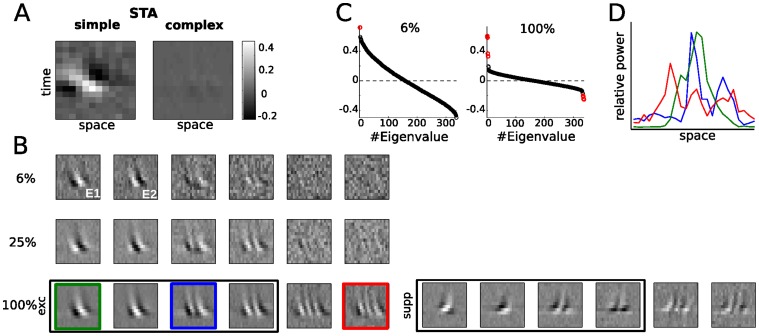
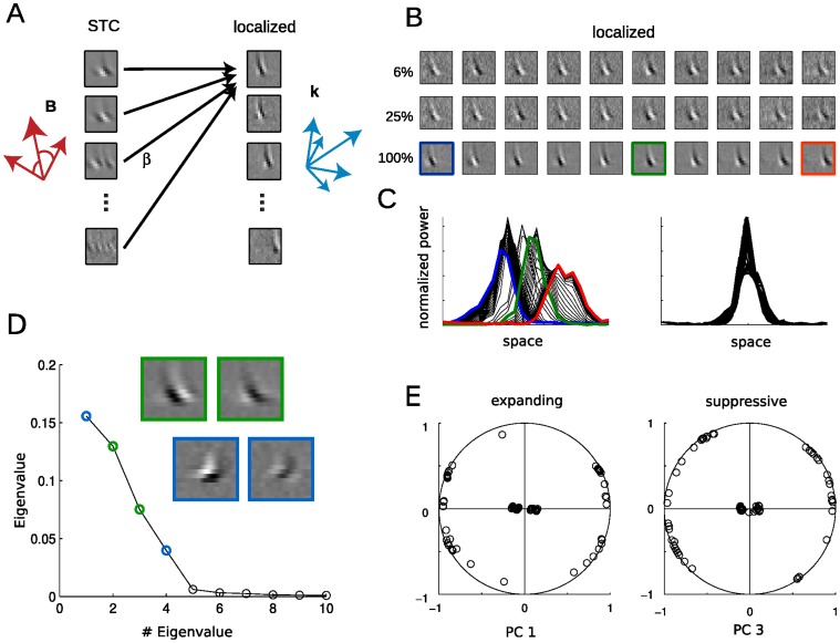
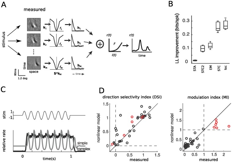
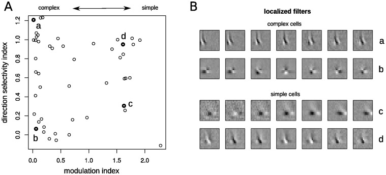
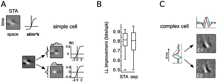
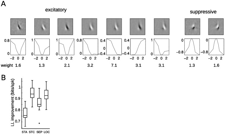
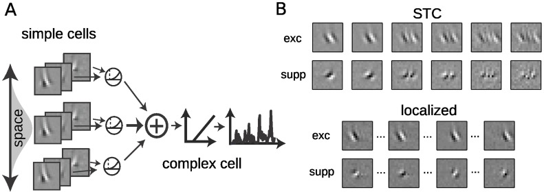
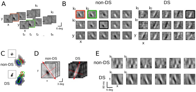
Despite detailed knowledge about the anatomy and physiology of neurons in primary visual cortex (V1), the large numbers of inputs onto a given V1 neuron make it difficult to relate them to the neuron's functional properties. For example, models of direction selectivity (DS), such as the Energy Model, can successfully describe the computation of phase-invariant DS at a conceptual level, while leaving it unclear how such computations are implemented by cortical circuits. Here, we use statistical modeling to derive a description of DS computation for both simple and complex cells, based on physiologically plausible operations on their inputs. We present a new method that infers the selectivity of a neuron's inputs using extracellular recordings in macaque in the context of random bar stimuli and natural movies in cat. Our results suggest that DS is initially constructed in V1 simple cells through summation and thresholding of non-DS inputs with appropriate spatiotemporal relationships. However, this de novo construction of DS is rare, and a majority of DS simple cells, and all complex cells, appear to receive both excitatory and suppressive inputs that are already DS. For complex cells, these numerous DS inputs typically span a fraction of their overall receptive fields and have similar spatiotemporal tuning but different phase and spatial positions, suggesting an elaboration to the Energy Model that incorporates spatially localized computation. Furthermore, we demonstrate how these computations might be constructed from biologically realizable components, and describe a statistical model consistent with the feed-forward framework suggested by Hubel and Wiesel.

Figure 1. Spike triggered analysis of direction selective simple and complex V1 cells.

A. The Spike Triggered Average (STA) for a simple cell (left) and a complex cell (right), shown as “x-t” plots: the horizontal axis corresponds to the spatial location perpendicular to a bar oriented in the neuron’s preferred direction, and the vertical axis indicates the time preceding a spike (10–140 ms). The grayscale value represents the magnitude of the STRF, indicating how strongly an increased/decreased luminance value at a spatiotemporal location increases or decreases the probability to spike. The tilt in the simple cell STA (left) demonstrates that it is direction selective, but the STA cannot capture the direction selectivity of the complex cell (right). B. V1 DS complex cells are sensitive to large numbers of motion features but the specific number of significant STC filters strongly depends on the amount of available data. With increasing data, more and more filters are detected (lines correspond to 8423, 28435, and 117097 spikes, respectively). However, the filters added (both “excitatory” and “suppressive”) with more data do not resemble those first detected, having higher spatial frequencies and less spatial localization (suppressive filters for smaller amounts of data are present but not shown). Note that the suppressive filters (bottom row, right) have opposite direction selectivity from the excitatory filters (left). The thin frame indicates the filters with the largest positive and negative eigenvalues, corresponding to the red dots in (C). C. The corresponding eigenvalue spectra of the spike-triggered covariance (STC) matrices estimated from 6% and 100% of the data indicate two vs. eight significant filters (red circles), respectively. D. The profiles of temporal power along each pixel position for the three STRFs indicated in B (last row) are diverse, ranging from relatively localized and unimodal to spatially extensive and multimodal.

Figure 2. Localized filters provide a biologically plausible alternative description of the STC subspace.

A. The subspace defined by the STC filters can be used to find a set of localized filters, where each localized filter (right) is a linear combination of the set of STC filters (left). The small filters (STC and localized) are taken from 1B and 2B (last row) and exemplify the different features that can be used to represent a cells sensitivity. Red arrows illustrate an orthogonal vector space defined by the STC filters, while blue arrows illustrate a larger number of non-orthogonal localized filters that span the same subspace. B. Localization detects a large number of filters within the STC subspace, and 10 (from 47) localized solutions spanning the RF are shown. As more data is used for the analysis, the properties of the filters remain relatively constant, but their features become less polluted by noise. The localized solutions show similar spatiotemporal sensitivity, with the main differences between the filters amounting to differences in position and phase. C. The power profiles of 47 localized excitatory filters (left) have been aligned (right) to compare the similarity of their spatial envelopes. D. The 47 excitatory and 47 suppressive localized solutions form 2 homogeneous populations of spatially confined features that are succinctly described by four eigenvectors - two spanning the excitatory subspace, and two spanning the suppressive subspace - as determined by PCA applied to the set of spatially shifted localized filters in D. E. The filters are well represented by these PCA eigenvectors (98% exp, 97% suppressive) and evenly cover the range of possible combinations of these vectors.

Figure 3. Nonlinear modeling predicts spike timing direction selectivity and modulation index for simple and complex cells.

A. Schematic of the nonlinear model structure. The stimulus is filtered by a set of receptive fields k_i and further processed by associated nonlinearities f_i(.) and temporal combination term h_{i .} Outputs of multiple expanding and suppressive modules are summed together and converted into a firing rate prediction r(t) via the spiking nonlinearity F. B. Cross-validated log-likelihood (LL) improvement compared to a model based on the average firing rate. The different levels of STC-based models demonstrate that models with two filters (STC2 and EM) offer large improvements in LL over a model based on the STA alone. However, including the full set of detected filters (STC and loc) more than doubles model performance. STC2 refers to the model containing only the first two STC filters shown in 1B, (last row), EM to the two STC filters found for small amounts of data (Fig. 1B , first row), STC to all filters shown in Fig. 1B (last row), and loc to the localized features (Fig 2B , last row). C. Simulated responses of a simple and a complex cell (model as shown in Figure 3A ) to optimally oriented drifting gratings demonstrate the ability of models fit to random bar stimuli to predict response properties to gratings consistent with their cell classification. The responses of the simple cell (gray) and complex cell (black) are shown relative to the temporal stimulus modulation at a given spatial location (top). D. Modulation index (MI) and direction selectivity measurements for 51 V1 cells stimulated with optimally oriented drifting gratings (Rust et. al. 2005). The models of all neurons in the study were used to generate predicted Direction Selectivity Index (DSI) and MI (vertical axis), which are in agreement with those values measured experimentally (horizontal axis), for simple (red, correlation coefficient CC = 0.93) and complex (black, CC = 0.84) cells, with CC = 0.85 overall. MI is predicted with similar fidelity (right, CC = 0.9).

Figure 4. Diversity of response properties across a population of simple and complex cells.

A. Empirically measured modulation index and direction selectivity values for 51 V1 cells (see Fig. 3, Rust et. al. 2005). The population contains simple and complex cells with varying degrees of direction selectivity. B. Both simple and complex cells display sensitivity consistent with multiple localized inputs (shown are 7 localized filters spanning the region RF of the individual cells indicated in A).

Figure 5. Construction principles of direction selectivity in prototypical simple and complex cells.

A. An example of a DS simple cell described by a single excitatory filter (left). A single nonlinearity associated with this filter, comprising an LN model, offers a good description of its observed response. lower right: An alternative model for the simple cell, comprised of two non-DS filters, each decomposable into spatial and temporal projections (profiles shown at left and top). Each non-DS filter has a rectifying nonlinearity associated with it (right), which is fit to the data. B. Performance of the two models of the simple cell from (A) are assessed by the log-likelihoods predicted for the left out samples in 10-fold cross-validation. The model based on separable non-DS filters (“sep”) yields comparable predictions, and thus provides a reasonable explanation of the simple cell’s DS. C. The two eigenvectors E1 and E2 corresponding to the two significant eigenvalues shown in Fig. 1B (top row) are both direction selective. Furthermore, they form a “quadrature pair”, and can be described by different combinations of the two sets of spatial (top) and temporal (left) kernels via the sum of two sets of separable filters, which are obtained using singular value decomposition. As shown in Adelson & Bergen (1989) and reflected in the data, 2 spatial and 2 temporal kernels suffice to form a quadrature pair. While this model performs significantly better than the STA it clearly misses the complex selectivity captured by the model containing multiple localized features (see crossvalidation performance shown in Fig. 3B ).

Figure 6. Localized features explain direction selectivity in representative simple cells.

A. The spike triggered analysis of a typical simple cell identifies multiple excitatory and suppressive filters. The top row shows the relevant localized STRFs from the excitatory (left) and suppressive (right) subspace and the lower row the associated nonlinearities. B. Although clearly a simple cell based on its modulation index (MI = 1.51), comparison of cross-validated likelihood indicates that the neuron is best described by multiple filters (“STC", “loc”). Models just based on the spike triggered average (“STA”, Fig. 5A ) or models replacing the excitatory filters by non-DS inputs (as in Fig. 5A ) yield lower performance.

Figure 7. Construction of DS complex cells by pooling over inputs from typical DS simple cells.

A. A complex cell model is constructed from a population of typical simple cell models having multiple excitatory and suppressive filters themselves. The family of simple cells is created by spatially shifting all filters of a prototypical simple cell model (see Fig. 6A) over a spatial envelope representing the complex cell receptive field. These inputs are summed and processed by a spiking nonlinearity to generate a firing rate prediction, and a Poisson spike generator then produces simulated data for further analysis. B. Upper panel: the STC filters for the simulated complex cell display a range of different spatiotemporal frequencies and opposing DS for excitatory and suppressive directions, as observed for all complex cells in this study (e.g., Fig. 1E). Lower panel: The localized features inferred from these STC directions comprise a set of homogeneous, spatially shifted units, which closely resemble the dominant excitatory and suppressive directions from the first-order model (Fig. 6A).

Figure 8. Receptive fields can be estimated from responses to naturalistic movies.

A. Two filters found by applying the STC and localization methods to a V1 complex cell recorded in the context of naturalistic movies. To represent the three dimensions of the filters (two spatial and one temporal), the filters are shown as a series of two-dimensional (2-D) spatial plots across latencies. B. The set of localized filters across space for an example non-DS neuron (14,664 spikes, DSI = 0.05, left) and DS neuron (2,628 spikes, DSI = 0.51, right). Here, each filter is represented by its 2-D spatial slice at 40 ms latency, which is the latency with maximal spatial power, i.e., variance across pixels (green and red outlined frames in A). The 15 spatial maps shown in each case are examples of localized filters centered on different spatial locations. C. A density plot showing the total temporal power across all localized filters for the non-DS (top) and DS (bottom) neurons, demonstrating that - despite using a range of locations for the localization method - localized filters only exist in a defined region. Rectangular insets indicate the relative size and position of the spatial filter, and the colored contours overlaid on density plot show the outline of three example localized filters. D. To compare with the results from the analysis on the random bars data (Figs. 1–5), spatiotemporal slices oriented in the neuron’s preferred direction (red arrows) are computed, and spatially projected on the axis perpendicular (red tick marks). E. Projections along the direction indicated in (D) for each neuron’s localized filters reveal x-t plots that are consistent with the 1-D dataset and illustrate differences in direction selectivity between the cells shown in (B) and (C).

References

1. Van Essen DC, Anderson CH, Felleman DJ (1992) Information processing in the primate visual system: an integrated systems perspective. Science 255: 419–423. - PubMed
1. Ringach DL, Shapley RM, Hawken MJ (2002) Orientation selectivity in macaque V1: diversity and laminar dependence. J Neurosci 22: 5639–5651. - PMC - PubMed
1. Jia H, Rochefort NL, Chen X, Konnerth A (2010) Dendritic organization of sensory input to cortical neurons in vivo. Nature 464: 1307–1312. - PubMed
1. Rust NC, Stocker AA (2010) Ambiguity and invariance: two fundamental challenges for visual processing. Curr Opin Neurobiol 20: 382–388. - PubMed
1. Movshon JA, Newsome WT (1996) Visual response properties of striate cortical neurons projecting to area MT in macaque monkeys. J Neurosci 16: 7733–7741. - PMC - PubMed
Publication types
LinkOut - more resources