Automated transmission-mode scanning electron microscopy (tSEM) for large volume analysis at nanoscale resolution

Abstract

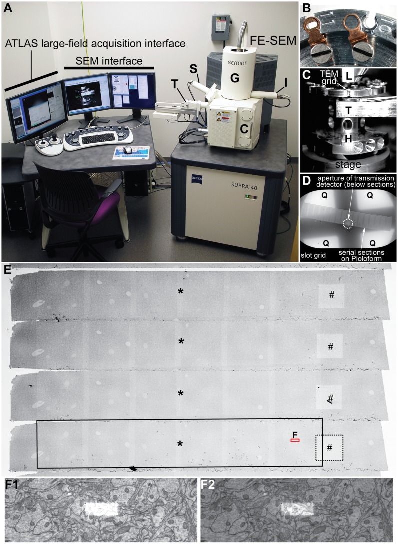
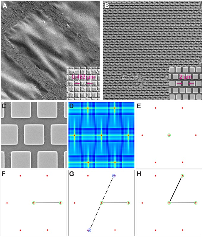
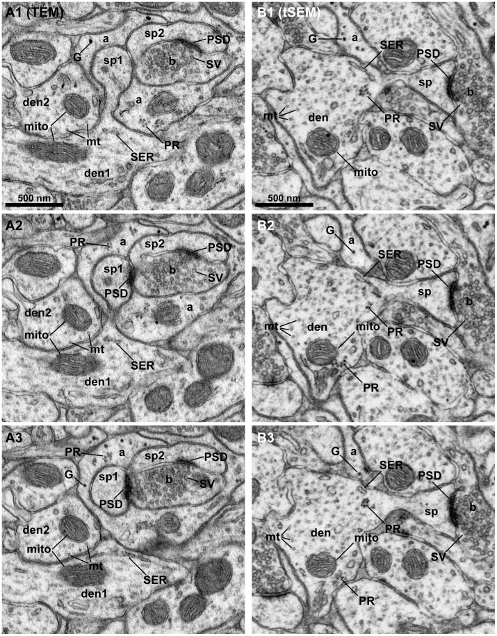
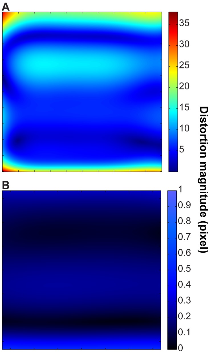
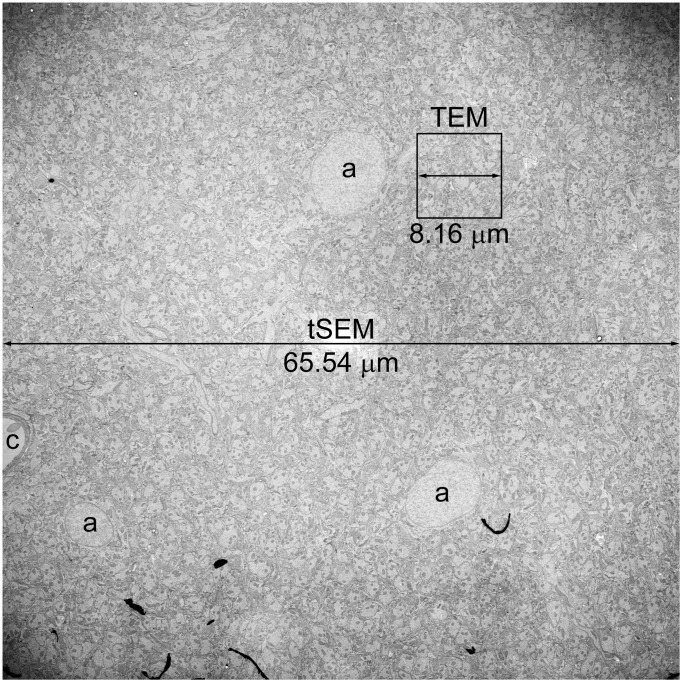
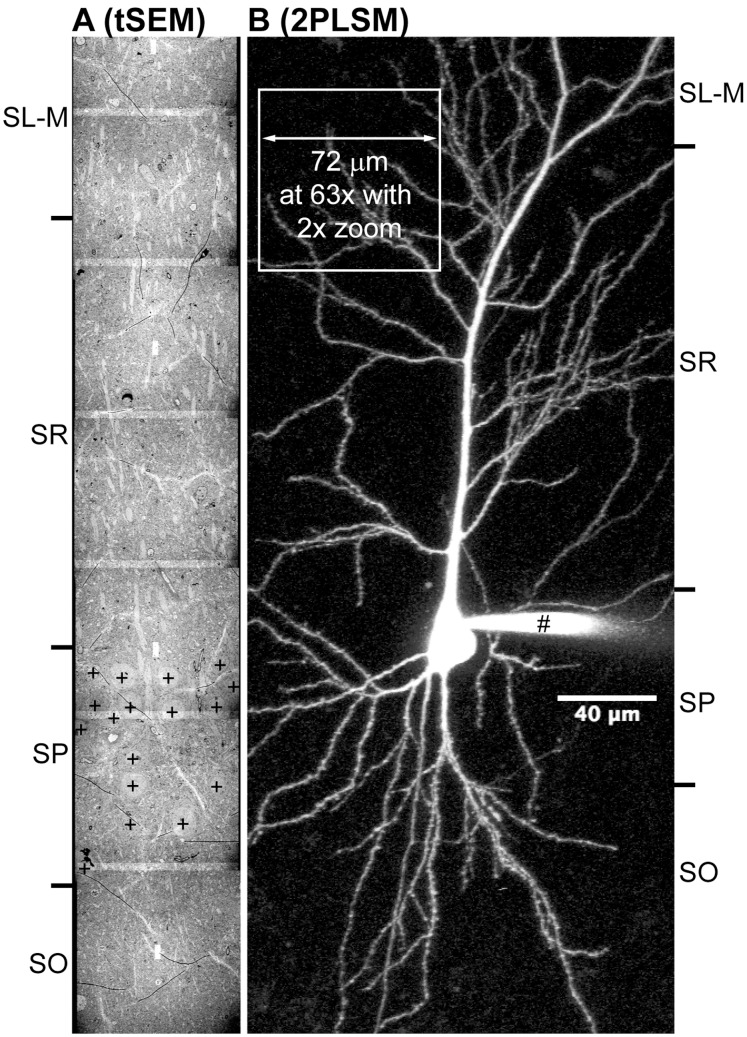
Transmission-mode scanning electron microscopy (tSEM) on a field emission SEM platform was developed for efficient and cost-effective imaging of circuit-scale volumes from brain at nanoscale resolution. Image area was maximized while optimizing the resolution and dynamic range necessary for discriminating key subcellular structures, such as small axonal, dendritic and glial processes, synapses, smooth endoplasmic reticulum, vesicles, microtubules, polyribosomes, and endosomes which are critical for neuronal function. Individual image fields from the tSEM system were up to 4,295 µm(2) (65.54 µm per side) at 2 nm pixel size, contrasting with image fields from a modern transmission electron microscope (TEM) system, which were only 66.59 µm(2) (8.160 µm per side) at the same pixel size. The tSEM produced outstanding images and had reduced distortion and drift relative to TEM. Automated stage and scan control in tSEM easily provided unattended serial section imaging and montaging. Lens and scan properties on both TEM and SEM platforms revealed no significant nonlinear distortions within a central field of ∼100 µm(2) and produced near-perfect image registration across serial sections using the computational elastic alignment tool in Fiji/TrakEM2 software, and reliable geometric measurements from RECONSTRUCT™ or Fiji/TrakEM2 software. Axial resolution limits the analysis of small structures contained within a section (∼45 nm). Since this new tSEM is non-destructive, objects within a section can be explored at finer axial resolution in TEM tomography with current methods. Future development of tSEM tomography promises thinner axial resolution producing nearly isotropic voxels and should provide within-section analyses of structures without changing platforms. Brain was the test system given our interest in synaptic connectivity and plasticity; however, the new tSEM system is readily applicable to other biological systems.

Figure 1. tSEM instrumentation.

A: Zeiss SUPRA 40 field emission scanning electron microscope equipped with a secondary electron detector (S), an in-lens detector (I), and a retractable detector for transmitted electrons (tSEM detector; T). The column (G) contains the gun assembly and objective lenses. The specimen chamber door (C) slides open outward with the stage. The SEM is controlled through the SEM interface and console of keyboard, mouse, joysticks, or the integrated ATLAS system for large-field imaging. The SEM can also be fitted with a backscatter electron detector (not shown). B: Top view of the specimen holder magnified to show two of the grid holding positions (10 and 11). Position 10 is empty and the copper clip is disengaged to the left of the slot, while position 11 contains a TEM grid (3 mm diameter) with the clip engaged. C: TV camera view of the specimen chamber showing the arrangement of the final lens (L), tSEM detector (T), and sample holder (H) on the stage. Working distance is 4–5 mm between the final lens and the specimen, and 4–5 mm between the specimen and the detector. Chamber vacuum is maintained at <10⁻⁷ Pa during imaging. D: Low-magnification tSEM image of an entire slot grid containing serial sections. Below the sections, the aperture of the tSEM detector can be seen (circle with dotted line), which must to be aligned to the center of the image field. Four quadrants (Q) of the detector element are also used for imaging by collecting electrons scattered at higher angles. Imaging mode (normal or inverted) can be set for each detector element on the SEM interface. E: SEM secondary electron image of another set of serial sections (different from that shown in D). Each section measures about 510 µm width×71 µm height. This image was taken after acquisition of two image series, one consisting of single frame images (32 µm×32 µm surrounding the #) and the other consisting of mosaic images (6 columns×1 row; 360 µm width×64 µm height, surrounding the *). These image fields are seen as brightened areas on each section (outlined by dotted and black boxes in the bottom section). Regardless of the target image size (single or mosaic field), the operator is required to mark only the center of each field (indicated by “#” or “*”,) to set up the serial image acquisition. The area outlined by a red box (“F”) is further magnified in F1–2. F1–2: Magnified view of a subfield measuring 10.8 µm×3.6 µm around the center of the image tile indicated in E. The brightened area in the center is where repeated scans took place during the autofocus routine. If the image brightness is adjusted to the entire field, the autofocus area becomes too bright to discern ultrastructure within this area (F1). As demonstrated in F2, however, these repeated scans during the autofocus routine do not cause loss of the underlying tissue structure. The original tSEM image was acquired as a 16-bit TIFF file at 2 nm pixel size. The image brightness was optimized for either the entire image field or the autofocus area to generate the images in F1 and F2. These images were then converted to 8-bit TIFF files and down-sampled to 12 nm pixel size for the final figure.

Figure 2. Distortion analysis method.

A: SEM secondary electron image of TEM calibration standard (crossed diffraction grating replica) on a 300-mesh grid. The grid is tilted at 20° shows a wrinkled surface (tilt axis = upper left to lower right, with some scan tilt correction applied). Image field is about 56 µm per side, as in figure A. Inset: Details of the grating replica. Note that each square measures 0.463 µm×0.463 µm. This tSEM image was taken without any tilt. B: SEM secondary electron image of an integrated circuit (IC) chip used for evaluation of SEM scan distortion. The chip is tilted at 65° (tilt axis = left to right, dynamically focused, no scan tilt correction applied) to illustrate flatness. Image field is about 56 µm per side, which is approximately the same size as tSEM images. Inset: Details of the IC chip. Note that each square-shaped element measures 2 µm×2 µm, and is arranged in hexagonal arrays. This SEM secondary electron image was taken without any tilt. C: SEM secondary electron image of IC chip as in A, cropped to correspond with illustrations in D–H. D: Energy map created from the normalized cross-correlation of an image of an individual IC unit with the original image. E: The energy map is thresholded and peaks selected from within the resulting connected components. For each peak, as shown encircled in green, we build a triplet model to use for rejecting false detections and for extracting the true regular pattern. F: The detected location is paired with its nearest neighbor to form a line segment. G: We form putative neighbor locations at expected angles above and below the line segment (+60° and −120°, respectively). H: Here, the distance to the detection closest to the upper putative neighbor was smaller than for the lower one. The upper neighbor is selected to complete the triplet.

Figure 3. Quality comparison of images acquired on tSEM vs. TEM.

Serial section images from the middle molecular layer of the hippocampal dentate gyrus acquired on a TEM (A1–3) and tSEM (B1–3). They were taken as 8-bit grayscale images, and the brightness and contrast were then adjusted to match the images from the two different EM platforms. A1–3: An obliquely cut dendrite (den1) gives rise to a mushroom-shaped spine (sp1) with postsynaptic density (PSD), making a synapse with an axonal bouton (b) containing synaptic vesicles (SV). This bouton also makes a synapse with another spine (sp2). These spines and bouton are wrapped around by an astrocytic process that contains glycogen granules (G) and polyribosomes (PR). A tubule of smooth endoplasmic reticulum (SER) and mitochondrion (mito) are located in the dendritic shaft. Cross-sectioned microtubules (mt) are clearly visible in an adjacent dendrite (den2), which also contains a mitochondrion (mito). B1–3: A mushroom-shaped spine (sp) on a dendrite (den) makes a synapse with a thickened PSD on an axonal bouton (b) containing synaptic vesicles (SV). A tubule of SER is visible at the base of this spine, along with a cluster of polyribosomes (PR). Cross-sectioned microtubules (mt) are also visible in this dendrite, which also contains a mitochondrion (mito). Clusters of polyribosomes (PR) are visible adjacent to a mitochondrion (in B2–3). Glycogen granules (G) are found in a neighboring astrocytic process (a). The original pixels are retained in all images in this figure. Only brightness and contrast were adjusted to match images acquired on the two EM platforms.

Figure 4. Image distortion analysis.

A: tSEM full field distortion magnitude, corresponding to 24,000×24,000 pixel image. Maximum distortion magnitude is 37.93 pixel (rms = 9.68 pixel). This is equivalent to 0.04% rms distortion. B: tSEM field in A was cropped to the size equivalent TEM field (4,096×4,096 pixels). Note the scale bar is necessarily different. Maximum distortion magnitude is 0.55 pixel (rms = 0.19 pixel). This is effectively zero distortion, equivalent to 0.0047% rms distortion. Since we cannot accurately measure stretch and shear in the calibration replica, we ignore affine distortion modes.

Figure 5. Field size comparison of images acquired on tSEM vs. TEM.

This single field image of the rat hippocampal dentate gyrus (inner molecular layer) was acquired on tSEM originally at 32,768×32,768 pixels, or 65.54 µm×65.54 µm at 2 nm/pixel. Three astrocyte soma with round nuclei (a) and part of a capillary (c) are visible in this image. Boxed area indicates the size of a single field that can be imaged on our TEM (4,080×4,080 pixels, or 8.16 µm×8.16 µm at 2 nm/pixel). Note that the size of TEM field is similar to that of the nucleus of an astrocyte. The image has been adjusted for brightness and contrast, and re-sampled from the original pixel dimensions to 1,836×1,836 pixels during preparation of this figure.

Figure 6. Field size comparison of images acquired on tSEM and two-photon laser-scanning microscope (2PLSM).

A: A tSEM image containing a mosaic of 7 image tiles, from rat hippocampal area CA1, with the field size measuring 67 µm×399 µm. Overlaps between image tiles appear as lighter bands. Soma of the pyramidal neurons are indicated by “+”. The original image tiles were taken as 10×1 mosaic covering 608 µm×65 µm area (32,768×32,768 pixels per tile at 2 nm pixel size), encompassing all layers in the area CA1 (SO = Stratum Oriens; SP = Stratum Pyramidale; SR = Stratum Radiatum; SL-M = Stratum Lacunosum Moleculare). The image tiles were stitched together with Fiji/TrakEM2, down-sampled to 223 nm pixel size, rotated 90°, and cropped to 303×1792 pixels (67 µm×399 µm) to scale with the image in B. B: A pyramidal neuron in the rat (10-week old) hippocampal area CA1 was filled with Alexa 594 dye (40 µM) with a patch pipette (#). The original fluorescence image stack was acquired using laser tuned to 880 nm (Spectra Physics Mai Tai) on a 2PLSM (Leica SP 5 RS) with a 20× water immersion objective (N.A. = 1.0). Image field size was 1024×1024 pixels (455.88 µm×455.88 µm and 120 µm deep; 255 optical sections), which was then projected and cropped to 384×896 pixels (171 µm×399 µm). White box indicates calculated field for imaging with a 63× objective and 2× digital zoom (i.e., 455.88 µm/[63/20]/2 = 72.36 µm), which is on the order of single field size of a tSEM image. Scale bar is valid for both A and B. Image courtesy of R. Chitwood, Center for Learning and Memory, The University of Texas at Austin.

References

1. Cook WR, MacAlister TJ, Rothfield LI (1986) Compartmentalization of the periplasmic space at division sites in gram-negative bacteria. J Bacteriol 168: 1430–1438. - PMC - PubMed
1. Keddie FM, Barajas L (1969) Three-dimensional reconstruction of Pityrosporum yeast cells based on serial section electron microscopy. J Ultrastruct Res 29: 260–275. - PubMed
1. Osafune T, Schwartzbach SD (2010) Serial section immunoelectron microscopy of algal cells. In: Schwartzbach SD, Osafune T, editors. Immunoelectron microscopy. Methods in molecular biology. Humana Press, Vol. 657: 259–274. - PubMed
1. Jarrell TA, Wang Y, Bloniarz AE, Brittin CA, Xu M, et al. (2012) The connectome of a decision-making neural network. Science 337: 437–444. - PubMed
1. Chiang RG, Govind CK (1986) Reorganization of synaptic ultrastructure at facilitated lobster neuromuscular terminals. J Neurocytol 15: 63–74. - PubMed
Publication types