Cortical-like receptive fields in the lateral geniculate nucleus of marmoset monkeys

Abstract

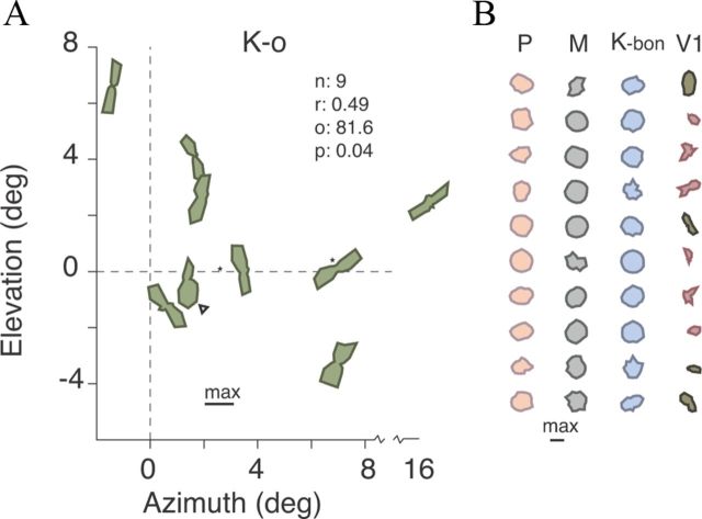
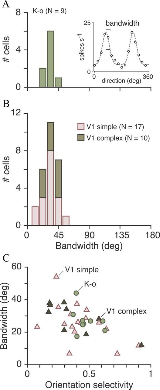
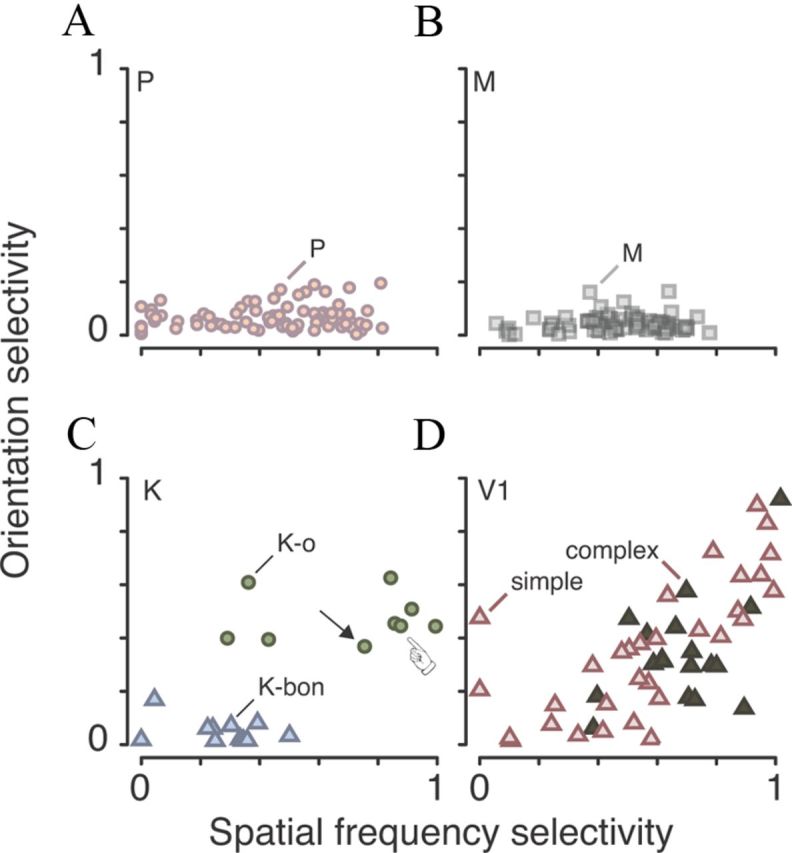
Most neurons in primary visual cortex (V1) exhibit high selectivity for the orientation of visual stimuli. In contrast, neurons in the main thalamic input to V1, the lateral geniculate nucleus (LGN), are considered to be only weakly orientation selective. Here we characterize a sparse population of cells in marmoset LGN that show orientation and spatial frequency selectivity as great as that of cells in V1. The recording position in LGN and histological reconstruction of these cells shows that they are part of the koniocellular (K) pathways. Accordingly we have named them K-o ("koniocellular-orientation") cells. Most K-o cells prefer vertically oriented gratings; their contrast sensitivity and TF tuning are similar to those of parvocellular cells, and they receive negligible functional input from short wavelength-sensitive ("blue") cone photoreceptors. Four K-o cells tested displayed binocular responses. Our results provide further evidence that in primates as in nonprimate mammals the cortical input streams include a diversity of visual representations. The presence of K-o cells increases functional homologies between K pathways in primates and "sluggish/W" pathways in nonprimate visual systems.

Figure 1.

Orientation and SF tuning of geniculate and cortical neurons. A–C, P cell. Top row (A), Orientation tuning curve of mean (F0) and fundamental harmonic (F1) responses. Gratings and arrows in A illustrate the stimuli presented on the monitor. Center row (B), PSTH folded to one cycle of the grating. Values above the PSTH indicate orientation of drift. Left, PSTH shows responses to optimal orientation. Right, PSTH shows orthogonal to optimal orientation. The P cell responds in phase to the stimulus. Lower row (C), SF tuning curve fit with the DOG model. The arrow indicates the SF at which the orientation tuning curve was measured. D–F, Orientation-selective cell responses, in the same format as A–C. This cell shows “simple-like” behavior with pronounced phase-locked F1 response (B). G–I, Second example of a K-o cell; this cell shows “complex-like” behavior with increased average firing (F0) for preferred orientations. J–L, Complex cell in primary visual cortex (V1). Note that the K-o cells and the complex cell show strong bandpass spatial tuning (F, I, L) and feeble responses to gratings drifting orthogonal to the preferred orientation (E, H, K). Error bars on graphs indicate SEM. Error bars are present at all data points but some are smaller than the point symbols.

Figure 2.

Distribution of orientation selectivity of geniculate and cortical cells. A, P cells. B, M cells. C, K-o cells. The gray bar shows a cell recorded in a K layer simultaneously with a K-bon cell. D, K-bon cells. E, Primary visual cortex (V1) simple cells. F, V1 complex cells. Orientation selectivity for K-bon cells was calculated from S-cone-isolating gratings. Orientation selectivity for all other cells was calculated from achromatic drifting gratings. Note the overlap in orientation selectivity between K-o and V1 cells.

Figure 3.

Orientation tuning and visual field location. A, Visual field map showing tuning curves (polar plots) of K-o cells. The center of each tuning curve is plotted at the visual field coordinates of the recorded cell. The curve of one K-o cell is displaced for clarity (asterisk). One cell (arrowhead) was recorded from the right LGN. The elongation on the y-axis of each tuning curve indicates greater responsivity to vertical orientations. Note that six of nine K-o cells prefer vertical orientations. n, number of cells; r, Rayleigh coherence of preferred orientations, o, mean of preferred orientations; p, probability value of Rayleigh coherence. Preferred direction was weighted by orientation selectivity for each cell in the coherence vector sum. B, Randomly selected samples of tuning curves of P, M, K-bon, and primary visual cortex (V1) cells. Note lack of strong tuning in P and M cells and lack of coherent preferred direction in V1 cells.

Figure 4.

Linear prediction of orientation bias. A, Orientation selectivity (OSI) as a function of relative SF. Relative SF was computed as the SF at which direction tuning was measured, divided by the preferred SF for each receptive field. K-o cells, n = 9; P cells, n = 73; M cells, n = 65. The contour lines show the linear predictions of OSI when orientation tuning is computed for concentric center-surround receptive fields of varying center aspect ratio (major-to-minor axis ratio, indicated at the end of each contour line). B, STA responses for achromatic white noise stimulus presented to two K-o cells. Grid bars indicate pixel borders. Pixel size (Pix:) is indicated below each graph. These K-o receptive fields show spatially separated On- and Off-subregions. The “hand” and arrow symbols indicate these cells in A. C, Temporal kernels for the pixels at the intersection of the border marks shown in B. Error lines indicate SDs. D, Linear prediction of direction tuning obtained by convolution of the STA with the direction tuning stimulus set. The tuning is consistent with the measured direction tuning (filled symbols). E, Left, STA response for a P cell, shown at the same spatial scale as the K-o cell. Right, Measured and predicted direction tuning for this cell. Note that measured and predicted direction selectivity is low.

Figure 5.

Orientation tuning bandwidth. A, Bandwidths (half-width at half-height) of K-o cells calculated from a bimodal wrapped normal fit of direction tuning curves (inset graph). B, Bandwidths of cortical (V1) cells. Note overlap of bandwidth with K-o cells. C, Scatterplot showing bandwidth and orientation selectivity (OSI). Note that for both K-o and V1 cells, tuning bandwidth sharpens as orientation selectivity increases, but narrow bandwidth is not essential for high orientation selectivity.

Figure 6.

Orientation and SF selectivity. Scatterplots of orientation selectivity and SF selectivity. Increasing values indicate greater selectivity. A, P cells (n = 79). B, M cells (n = 65). C, K-o cells (n = 9) and K-bon cells (n = 11). D, Cortical (V1) cells: simple cells (n = 31); complex cells (n = 18). Orientation selectivity for K-bon cells was calculated from S-cone-isolating gratings. Orientation selectivity for other cells was calculated from achromatic drifting gratings. The “hand“ and arrow symbols indicate the cells shown in Fig. 4B–D.

Figure 7.

Receptive field center diameter of geniculate and cortical neurons. Receptive field center diameter was calculated as twice the DOG model fit radius. A, P cells (n = 64). B, M cells (n = 21). C, K-o cells (n = 8) and K-bon cells (n = 25). D, Cortical (V1) cells: simple cells (n = 20); complex cells (n = 9). Note that receptive field size increases as a function of eccentricity for P and M cell cells. K-o cells tend to have smaller center sizes than BON cells. V1 neurons have center sizes encompassing the range of LGN neurons. Recordings from V1 cells were limited to the central 10°.

Figure 8.

Contrast tuning curves of geniculate and cortical neurons. A, Individual tuning curves for P cells. B, M cells. C, K-bon cells. D–F, Averaged normalized tuning curves for each class. The P cells and K-bon cells show linear contrast tuning; M cells show response saturation. G, Individual tuning curves for K-o cells. H, Cortical (V1) simple cells. I, V1 complex cells. J–L, Averaged normalized tuning curves for each class. The K-o cells show linear contrast tuning, V1 cells show saturating responses. Orientation selectivity for K-bon cells was calculated from S-cone-isolating gratings. Orientation selectivity for other cells was calculated from achromatic drifting gratings. Contrast is referred to maximum achievable with the monitor (80% for S-cone-isolating gratings, >95% for achromatic gratings). Error bars indicate SEM. Many error bars are smaller than the data symbols.

Figure 9.

TF tuning curves of LGN and V1 cells. A, Individual tuning curves for P cells. B, M cells. C, K-bon cells. D–F, Averaged normalized tuning curves for each class. G, Individual tuning curves for K-o cells. H, Cortical (V1) simple cells. I, V1 complex cells. J–L, Averaged normalized tuning curves for each class. The M cells show the highest preferred TF, 16.03 ± 0.98 Hz (mean ± SEM); P cells, 7.58 ± 0.32; K-bon cells, 6.49 ± 1.43; K-o cells 9.28 ± 4.28; V1 simple cells, 6.20 ± 0.82; V1 complex cells,7.26 ± 1.10. Temporal selectivity indices are as follows: M cells, 0.60 ± 0.02; P cells, 0.47 ± 0.01; K-bon cells, 0.33 ± 0.06; K-o cells, 0.35 ± 0.12; V1 simple cells, 0.58 ± 0.06; V1 complex cells, 0.38 ± 0.05. Tuning curves for K-bon cells were calculated from S-cone-isolating gratings. Orientation selectivity for other cells was calculated from achromatic drifting gratings. Error bars indicate SEM. Many error bars are smaller than the data symbols.

Figure 10.

Binocular input to K-o cells. A, Orientation tuning curve of a K-o cell for gratings presented to the contralateral (right) eye. Dashed line shows amplitude of maintained activity. Error bars indicate SEM. B, PSTH for preferred orientation. Inset shows example spike waveforms. C, PSTH for orthogonal-to-preferred grating. D–F, Show responses in the same format, for gratings presented through the ipsilateral (left) eye. Note that the spike waveforms in B and E are indistinguishable, indicating recording from the same neuron. The orientation selectivity (OSI) for contralateral eye stimulation was 0.45; OSI for ipsilateral eye stimulation was 0.17. Stimulus parameters were as follows: contrast 1, SF 1.5 cyc deg⁻¹, TF 5 Hz, stimulus diameter 5°. G–I, Example of binocular facilitation in a second K-o cell. PSTHs show response to a brief (200 ms), white circular uniform stimulus (size 12°). Stimulus duration is represented by the trace below each histogram. Response to stimulation through both eyes (binoc) is greater than response to stimulation through the ipsilateral eye alone (ipsi) or contralateral eye alone (contra). Scale bar: (in I) G–I, 1 ms.

Figure 11.

Objective classification of K-o cells. A, B, Principal component analysis and objective clustering. The scatterplot shows first and second principal components derived from the following receptive field metrics, as described in the text: TFI, SFI, OSI, contrast sensitivity (half-saturation constant, C50), receptive field center radius (RC). The distribution of cell populations on these metrics is show in A. The vector projection of each metric on the principal component plane is shown in B. Note that K-o cells form a distinct cluster; the other cell groups (K-bon, M, P) form partially overlapping clusters. The “target” symbols in B show the centroid positions of four clusters in this dataset derived from k-means clustering. The centroid of cluster four corresponds to the position of K-o cells.

Figure 12.

Electrode track reconstruction of K-o cells. A, Micrograph of a coronal section stained for Nissl substance to reveal the cell layers of the LGN. B, Micrograph of the neighboring section showing electrode track revealed by autofluorescence. Arrowhead indicates an electrolytic lesion (+5 μA, 5 s). Autofluorescent tracks and lesions, together with changes in eye dominance and functional cell properties, were used to align the micrographs with the microdrive depths of recorded cells. C, Schematic representations of these sections showing geniculate layers, electrode track, and recorded cells. K-o cells are indicated by red symbols and arrowheads. The star in D indicates the K-o cell described in Figure 10A–C.

Figure 13.

Summary of K-o cell recording positions. Closed symbols represent cells whose recording positions were anatomically reconstructed. Open symbols represent cells whose positions were inferred from physiological measures.

References

1. Alitto HJ, Moore BD, 4th, Rathbun DL, Usrey WM. A comparison of visual responses in the lateral geniculate nucleus of alert and anaesthetized macaque monkeys. J Physiol. 2011;589:87–99. doi: 10.1113/jphysiol.2010.190538. - DOI - PMC - PubMed
1. Alonso JM, Usrey WM, Reid RC. Precisely correlated firing in cells of the lateral geniculate nucleus. Nature. 1996;383:815–819. doi: 10.1038/383815a0. - DOI - PubMed
1. Benevento LA, Yoshida K. The afferent and efferent organization of the lateral geniculo-prestriate pathways in the macaque monkey. J Comp Neurol. 1981;203:455–474. doi: 10.1002/cne.902030309. - DOI - PubMed
1. Berens P. CircStat: a MATLAB toolbox for circular statistics. J Stat Software. 2009;31
1. Bishop PO, Burke W, Davis R. The interpretation of the extracellular response of lateral geniculate cells. J Physiol. 1962;162:451–472. - PMC - PubMed
Publication types
LinkOut - more resources