When is it time to move to the next raspberry bush? Foraging rules in human visual search

Abstract

Animals, including humans, engage in many forms of foraging behavior in which resources are collected from the world. This paper examines human foraging in a visual search context. A real-world analog would be berry picking. The selection of individual berries is not the most interesting problem in such a task. Of more interest is when does a forager leave one patch or berry bush for the next one? Marginal Value Theorem (MVT; Charnov, 1976) predicts that observers will leave a patch when the instantaneous yield from that patch drops below the average yield from the entire "field." Experiments 1, 2, 3, and 4 show that MVT gives a good description of human behavior for roughly uniform collections of patches. Experiments 5 and 6 show strong departures from MVT when patch quality varies and when visual information is degraded.

Keywords: decision rules; foraging; marginal value theorem; visual attention; visual search.

Figure 1

A Massachusetts blueberry farm would like you to search exhaustively even if Optimal Foraging Theory predicts otherwise. Reprinted by permission of Turkey Hill Farm, Haverhill, MA 01830.

Figure 2

Stimulus configuration for Experiment 1: Modified screenshot.

Figure 3

RT as a function of the “reverse click order.” Click 1 is the final click in a patch. HF = Hard, Fast condition; HS = Hard, Slow; EF = Easy, Fast; ES = Easy, Slow. Solid lines are averages of nine observers. Error Bars show ±1 SEM.

Figure 4

Picked berry color as a function of the “forward click order.” Here, position 1 is the first click in the patch.

Figure 5

Positive predictive value (PPV) of each click, averaged from the final click in a patch. In this case, PPV = “good” berries/berries picked.

Figure 6

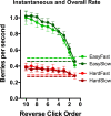
Instantaneous (solid lines) versus overall (dashed) rates of return four each of the four conditions of Experiment 1. Error bars = ±1 SEM.

Figure 7

z(Hit) as a function of z(False Alarm) for each subject in each condition of Experiment 2. Note that this is a portion of the ROC space. The d' = 0 line is shown in the lower right.

Figure 8

Rate (berries/s) for the last seven berries picked in each condition. Here those last clicks are plotted against time since the start of picking in that patch. Error bars are ±1 SEM.

Figure 9

Screen shot of stimuli for Experiment 3.

Figure 10

Average (± SEM) instantaneous rate for the final nine clicks for each of the four conditions of Experiment 3. Dashed lines show average rate of return for each condition. Slow travel conditions are shown with outlined symbols and coarsely dashed lines for the average rate.

Figure 11

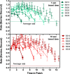
Rate of return for the last seven berries picked as a function of the time in the patch for that selection. Data are averaged over all observers and set sizes. Error bars are ±1 SEM. Slower travel (dark red) leads to longer time in each patch than fast travel (light green). In the fast travel condition, observers leave the patch when the rate reaches the average rate (dashed line). However, in the slow travel condition, observers leave the patch well before they reach the average rate.

Figure 12

Rate of return as a function of set size. Averages work backward from the final berry picked in a patch. Data are averaged over all observers with different brightness/color lines showing different set sizes. Error bars are ±1 SEM. The upper panel shows the fast travel condition, and the lower panel shows the slow condition. Dashed lines show the average rate of return for the block.

Figure 13

Instantaneous rate as a function of time in patch. Data averaged over 10 observers for the last 10 selections. Dashed lines show average rates for the fast (light green) and slow (dark red) blocks.

Figure 14

Instantaneous rate as a function of time in patch shown for each level of patch quality (probability that a berry is a good berry). Data averaged over 10 observers relative to the last selection in the patch. Dashed lines show average rates for the fast and slow travel time blocks.

Figure 15

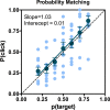
Probability of clicking on a “berry” as a function of the probability that a given berry is a target (patch quality). Filled green symbols show individual observer data for travel time of 1 s. Open green circles show the average of those data. Solid black line is the linear regression of those data. Dashed purple line shows the linear regression for travel time of 10 s. The dotted line has a slope of 1.0, representing perfect probability match behavior.

Figure 16

Rate in berries per second as a function of average time in patch for Experiment 6. Different curves represent different probabilities of a “good” berry. Points are plotted for those conditions where there was such a click for 75% of patches, across observers.

Figure 17

Probability of selecting an item P(click) as a function of the probability that the item will be a target (patch quality, P[target]). Smaller, paler data points represent individual observers. Large, dark points show average data. The solid line is the best-fit regression line. It is very close to the dashed line, showing the predictions of perfect probability matching.

Figure 18

False alarms (bad berries) per patch as a function of patch quality.

References

1. Beck V. M., Hollingworth A., Luck S. J. (2012). Simultaneous control of attention by multiple working memory representations. Journal of Vision, 12 (9), 956, http://www.journalofvision.org/content/12/9/956, doi:10.1167/12.9.956. [Abstract] - PMC - PubMed
1. Bond A. B., Kamil A. C. (2002). Visual predators select for crypticity and polymorphism in virtual prey. Nature, 415 (6872), 609–613. - PubMed
1. Cain M. S., Vul E., Clark K., Mitroff S. R. (2011). A Bayesian optimal foraging model of human visual search. Psychological Science, 23, 1047–1054, doi:doi:10.1177/0956797612440460. - DOI - PubMed
1. Charnov E. L. (1976). Optimal foraging, the marginal value theorem. Theoretical Population Biology, 9, 129–136. - PubMed
1. Eckstein M. P. (2011). Visual search: A retrospective. Journal of Vision, 11 (5): 10 1–36, http://www.journalofvision.org/content/11/5/14, doi:10.1167/11.5.14. [PubMed] [Article] - PubMed
Publication types
LinkOut - more resources