Measuring EGFR separations on cells with ~10 nm resolution via fluorophore localization imaging with photobleaching

Abstract

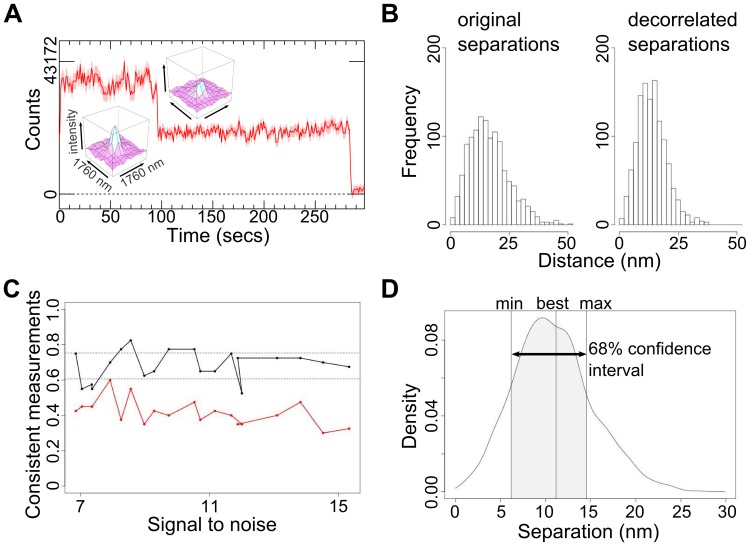
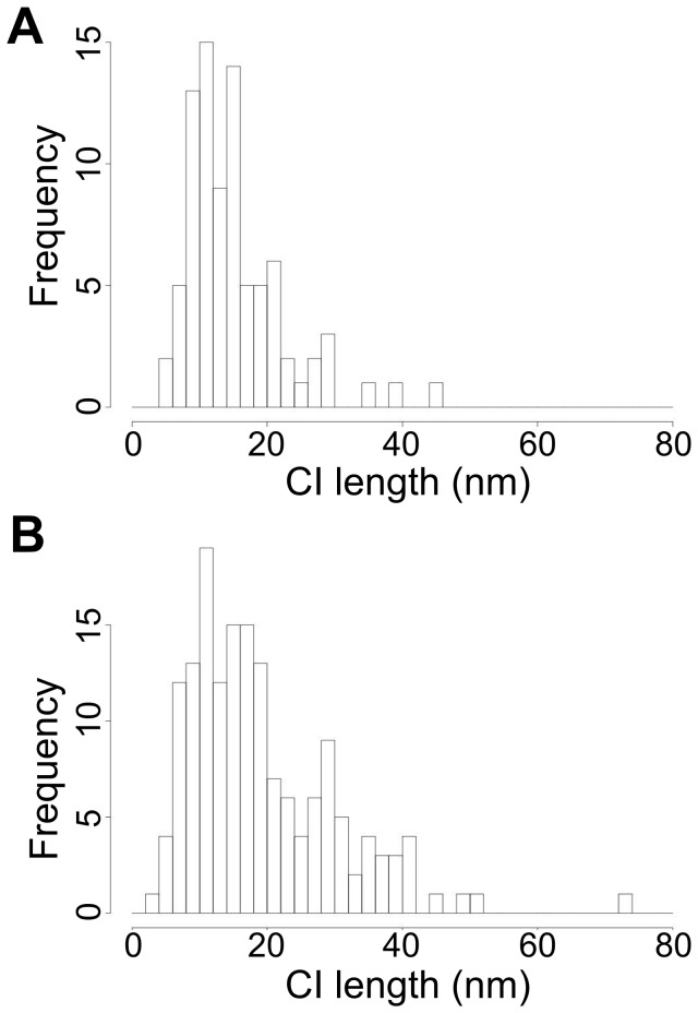
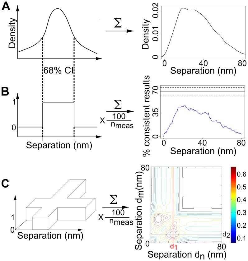
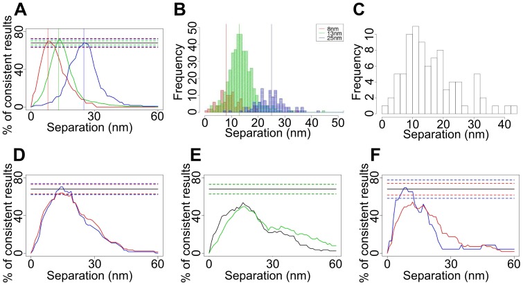
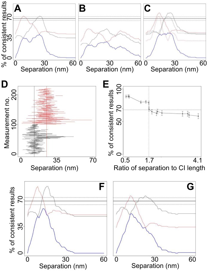
Detecting receptor dimerisation and other forms of clustering on the cell surface depends on methods capable of determining protein-protein separations with high resolution in the ~10-50 nm range. However, this distance range poses a significant challenge because it is too large for fluorescence resonance energy transfer and contains distances too small for all other techniques capable of high-resolution in cells. Here we have adapted the technique of fluorophore localisation imaging with photobleaching to measure inter-receptor separations in the cellular environment. Using the epidermal growth factor receptor, a key cancer target molecule, we demonstrate ~10 nm resolution while continuously covering the range of ~10-80 nm. By labelling the receptor on cells expressing low receptor numbers with a fluorescent antagonist we have found inter-receptor separations all the way up from 8 nm to 59 nm. Our data are consistent with epidermal growth factor receptors being able to form homo-polymers of at least 10 receptors in the absence of activating ligands.

Figure 1. Measuring the separation between two molecules.

(A) Example intensity v time course from a spot on cells showing a pair of Affibody-Atto 647N molecules photobleaching in two steps. Images were acquired every 0.28 s. The insets show the profile of the spot before and after the first bleaching event. (B) Original and decorrelated separations to illustrate the effect of anti-correlated positional error. The data of each spot is resampled and fitted 1200 times yielding 1200 sets of seven parameters that are samples of the 7-dimensional parameter distribution. In the decorrelated version the parameters have been independently randomly reordered, i.e. parameters from the same set end up in different sets. (C) Comparison of the error estimation of the Thompson, Larson and Webb and sequential photobleaching NALMS analysis method (red line) to our FLIP variant (black line) for synthetic data, depending on the SNR. SNR is the ratio of the measured mean intensity of a single-fluorophore trace to its standard deviation. The graph shows how often the real distance lies within the 68% confidence interval of the measurement. For , the confidence interval was taken as separation estimate ± standard deviation; for FLIP the confidence interval was taken as the shortest interval that contains 68% of the separation results from the bootstrap sampling (1,200 samples per measurement). (D) A probability density plot of the separations from the bootstrap samples of an individual measurement, showing the best fit value and the confidence interval.

Figure 2. Examples of observed large (left) and small (right) sample drifts.

The plots show a combined aligned track for the drift in position (pixels) in X (solid red line) and Y (solid green line) from all tracks in a set of images. The fitted global drift of the sample, a quadratic model fitted using ordinary least squares, is shown as a blue line for X and lilac for Y.

Figure 3. Comparing single molecule TIRF images from glass-immobilised molecules and from cells.

(A) Single-molecule TIRF image of glass-immobilised 13.3 nm DNA rulers, labelled at each end with Atto 647 N. (B) Single-molecule TIRF image of T47D cells labelled with anti-EGFR Affibody-Atto 647 N. Scale bar = 8 µm.

Figure 4. How close a second spot can be without affecting the calculated separation.

Simulations to determine how close, using distances in the range 3–8 pixels (as indicated to the left or right of each plot), a second spot can be before it affects the calculated separation within the first spot. If it is closer than 7 pixels (FWHM of the spot is 3 pixels), the separation is miscalculated and the percentage of consistent measurements does not reach 68%. Each plot shows data from 30 tracks. The simulated separation is 13 nm.

Figure 5. Distribution of the length of the confidence intervals.

(A) From experimental data from the 13.3 nm DNA ruler immobilised in glass. (B) From EGFR-Affibody on the surface of T47D cells.

Figure 6. Using confidence intervals as diagnostics.

(A) A sum of the individual bootstrap separation densities. The left-hand side shows a cartoon of the separation distribution of a single two-fluorophore spot. The right-hand side shows the distribution of the combined separation data from multiple two-fluorophore spots. (B) A _1sCI-Plot (right) is the scaled sum of top hat functions (left). Each top hat is created from the bootstrap separation distribution of a two-fluorophore spot. The top hat - or indicator - function has the value 1 if the separation lies within the 68% confidence interval, otherwise it has the value 0. The _1sCI-Plot plot (right) is an example sum of such functions for multiple two-fluorophore spots, where the scaling consists of dividing by the number of spots and then multiplying by 100 for a % scale. Hence, a value of 50% at a particular separation means that separation lies in the 68% confidence interval of the separation distribution of half of the two-fluorophore spots included in the analysis. The black line shows the ideal peak value (68%) expected for a repeated measurement of a single distance and the dashed lines show the uncertainty of this ideal due to the limited number of samples. (C) A _2sCI-Plot is the scaled sum of crosses, all with the same height and with equal arm widths given by the 68% confidence limits of each individual bootstrapped separation.

Figure 7. Population-averaged single-distance separations.

(A) _1sCI-Plots for simulated separations of 8 nm (red), 13 nm (green) and 25 nm (blue). The true distances are indicated by vertical lines. (B) Histogram of best fits for the 8, 13 and 25 nm simulated data. The calculated separation values from the best fits are 9.6±0.5 nm, 13.9±0.3 nm and 25.1 nm (C) Histogram of best fits and (D) _1sCI-Plots for the 13.3 nm DNA ruler data showing data sets where the root mean square of the residuals from fitting to the drift model exceeded 0.04 pixels (6.4 nm) were included (red) and excluded (blue). (E) _1sCI-Plots for end-to-end distance measurements of 8 nm (black) and 13.3 nm (green) DNA rulers without drift correction. The drift of the sample as a whole makes the distance appear larger and less defined. (F) 8 nm DNA rulers, showing data sets where the root mean square of the residuals from fitting to the drift model exceeded 0.04 pixels (6.4 nm) were included (red) and excluded (blue).

Figure 8. Multiple-distance separations.

(A) _1sCI-Plots (blue) and cross-sections through the _2sCI-Plots (black and red cross-sections, as shown in Fig. 6C) for mixes of simulated datasets with 8 and 25 nm separations. (B) Same as (A) for mixes of 8, 25 and 45 nm separations. (C) Same as (A) for mixes of 13 and 25 nm separations. The solid and dotted lines in correspond to all data and data with CI ≤7 nm respectively. (D) CIs of the simulated mixed 13 nm (black) and 25 nm (red) separations. The six marks show some confidence intervals that miss the correct separation, but hit the other separation. These false positives mean more CIs than expected seem to agree with the 13 nm-25 nm separation pair and the peaks in Fig. 8C exceed 68%. CIs that contain both separations are true positives. (E) Relation between the average CI length and the resolution. For different pairs of distances in simulated data sets, the maximal percentage of consistent measurements in the _2sCI-Plot is plotted against the ratio of separation to CI length. If the separation of the two distances is small compared to the length of the confidence intervals the CI-Plot has high peaks, indicating that the distances could not be resolved. If the separation between the two distances is larger than 1.7 times the average CI length, then the CI-Plot shows a maximum of around 68% consistent measurements. That indicates that the distances could be resolved. (F) _1sCI-Plots (blue) and cross-sections through the _2sCI-Plots (black and red) for mixes of simulated datasets 8 and 13 nm separations and (G) 8, 13 and 25 nm separations. The numbers of datasets with 8, 13, 25 and 45 nm separation were 100, 420, 120 and 60 respectively.

Figure 9. EGFR Affibody molecule does not activate the receptor.

(A) Western blots of A431 cell immunoprecipitates (I) and whole cell lysates (C) from unstimulated cells (blank) and cells stimulated with either 100 nM EGF or 2 nM EGFR Affibody. Proteins were probed (left to right) for non-specific tyrosine phosphorylation of proteins (Anti-pY4G10), tyrosine phosphorylation of EGFR (Anti-pY1045 EGFR) to show activated receptor, and presence of EGFR (Anti-EGFR). (B) Results of densitometry normalized against the total EGFR and relative quantity expressed as a fold change compared to an unstimulated control.

Figure 10. Separations of surface HER1-Affibody complexes in T47D cells.

(A) Separation distribution formed by summing 121 individual separation density functions. (B) The corresponding _1sCI-Plot (blue) and (C) cross-sections through the _2sCI-Plot (black and red). (D) Separation distribution formed by summing the 79 individual separation density functions with CIs ≤20 nm. (E) The corresponding _1sCI-Plot (blue) and (F) cross-sections through the _2sCI-Plot (black and red). (G) Separation distribution formed by summing the 24 individual separation density functions with CIs ≤10 nm. (H) Histogram of best fits for the data in (G). (I) Model of EGFR homo-polymer that can explain the distances derived from (G).

References

1. Lemmon MA, Schlessinger J (2010) Cell signaling by receptor tyrosine kinases. Cell 141: 1117–1134. - PMC - PubMed
1. Ferguson KM, Berger MB, Mendrola JM, Cho HS, Leahy DJ, et al. (2003) EGF activates its receptor by removing interactions that autoinhibit ectodomain dimerization. Mol Cell 11: 507–517. - PubMed
1. Garrett TP, McKern NM, Lou M, Elleman TC, Adams TE, et al. (2002) Crystal structure of a truncated epidermal growth factor receptor extracellular domain bound to transforming growth factor alpha. Cell 110: 763–773. - PubMed
1. Ogiso H, Ishitani R, Nureki O, Fukai S, Yamanaka M, et al. (2002) Crystal structure of the complex of human epidermal growth factor and receptor extracellular domains. Cell 110: 775–787. - PubMed
1. Zhang X, Gureasko J, Shen K, Cole PA, Kuriyan J (2006) An allosteric mechanism for activation of the kinase domain of epidermal growth factor receptor. Cell 125: 1137–1149. - PubMed
Publication types