The benefits of selecting phenotype-specific variants for applications of mixed models in genomics

Abstract

Applications of linear mixed models (LMMs) to problems in genomics include phenotype prediction, correction for confounding in genome-wide association studies, estimation of narrow sense heritability, and testing sets of variants (e.g., rare variants) for association. In each of these applications, the LMM uses a genetic similarity matrix, which encodes the pairwise similarity between every two individuals in a cohort. Although ideally these similarities would be estimated using strictly variants relevant to the given phenotype, the identity of such variants is typically unknown. Consequently, relevant variants are excluded and irrelevant variants are included, both having deleterious effects. For each application of the LMM, we review known effects and describe new effects showing how variable selection can be used to mitigate them.

Figure 1. The effects of excluding relevant SNPs and including irrelevant SNPs on phenotype prediction.

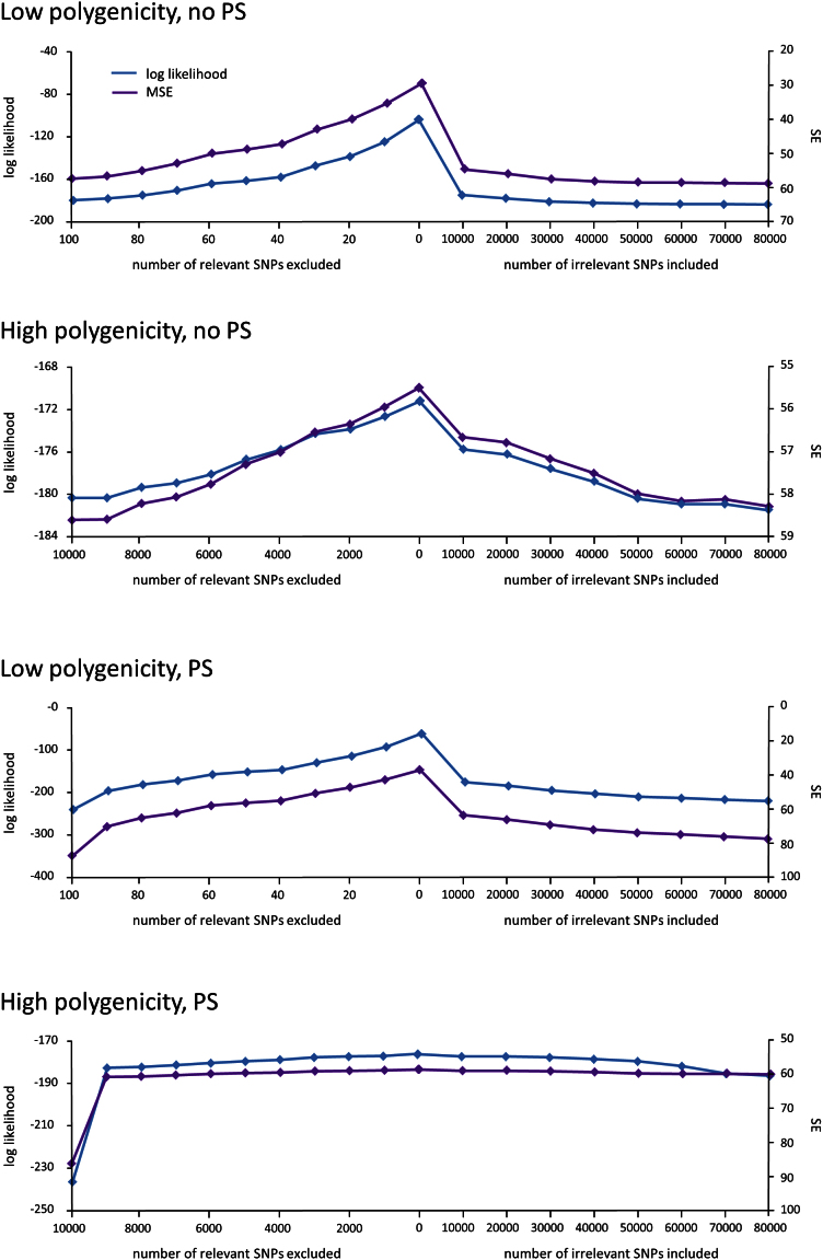
Out-of-sample log likelihood (blue) and squared error (purple) averaged over the folds of cross validation are plotted as a function of the number of relevant SNPs randomly excluded (left) and number of irrelevant SNPs randomly included (right) in the RRM.

Figure 2. Variable selection for phenotype prediction.

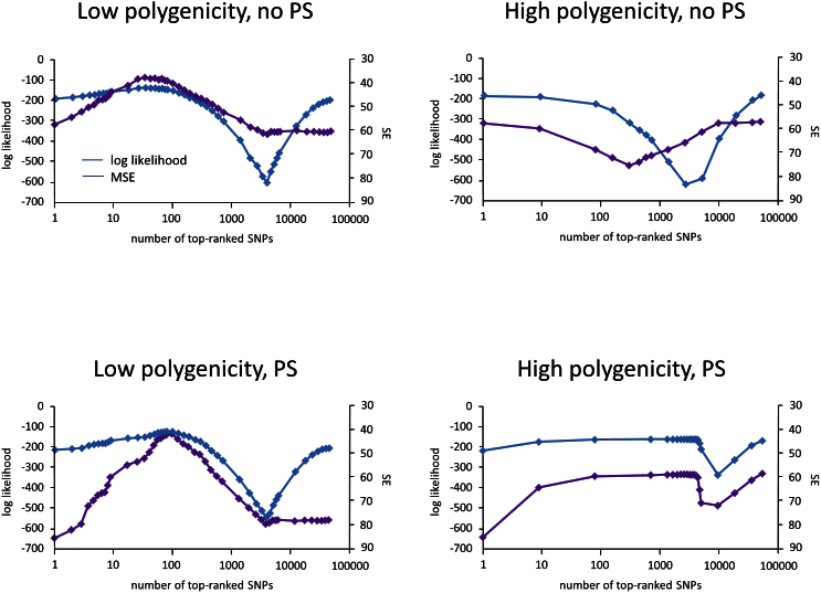
For each fold in 10-fold cross-validation, SNPs are sorted by their univariate P values on the training data. Then, the top k SNPs are used to train the LMM. Finally, the out-of-sample log likelihood and squared error are computed using the LMM and averaged over the folds. The plots show the averaged log likelihood (blue) and squared error (purple) as a function of k.

Figure 3. The effects of excluding relevant SNPs and including irrelevant SNPs on power and inflation.

(a) AUC as a function of the number of the causal SNPs excluded (with no irrelevant SNPs included), the number of differentiated SNPs excluded (with no irrelevant SNPs included), and the number of irrelevant SNPs included for the low and high polygenicity cases (including all relevant SNPs). (b) The genomic control factor λ as a function of the number of causal SNPs excluded (with no irrelevant SNPs included), the number of differentiated SNPs excluded (with no irrelevant SNPs included), and the number of irrelevant SNPs included for the high polygenicity case (including all relevant SNPs). The performance of the simple variable-selection method is indicated with green lines. The only plot with a non-monotonic pattern is the one showing λ as a function of the number of causal SNPs excluded (lower left). Nonetheless, the effect is significant in that, with 6,000 or more causal SNPs excluded, the GWAS P value distributions differ significantly from uniform according to a two-sided KS test (P values 0.047, 0.021, and 0.002 for 6,000, 8,000, and 10,000 SNPs excluded, respectively).

Figure 4. Number of associated methylation loci in the four brain regions (TCTX, FCTX, CRBLM, and PONS) that pass a Bonferroni-corrected P value threshold of 0.05 as a function of DNA sequence window size.

Only methylation loci that had at least one SNP in every window were included in the analysis so as to make the windows comparable. The plots are divided into those for even (a) and odd (b) chromosomes.

References

-
- Goddard M. E., Wray N. R., Verbyla K. & Visscher P. M. Estimating Effects and Making Predictions from Genome-Wide Marker Data. Statistical Science 24, 517–529 (2009).
- Yu J., Pressoir G., Briggs W. H., Vroh Bi I., Yamasaki M., Doebley J. F., McMullen M. D., Gaut B. S., Nielsen D. M. & Holland J. B. et al. A unified mixed-model method for association mapping that accounts for multiple levels of relatedness. Nature Genetics 38, 203–208 (2006). - PubMed
Publication types
MeSH terms
Grants and funding
LinkOut - more resources
Full Text Sources
Other Literature Sources