Unravelling daily human mobility motifs

Abstract

Human mobility is differentiated by time scales. While the mechanism for long time scales has been studied, the underlying mechanism on the daily scale is still unrevealed. Here, we uncover the mechanism responsible for the daily mobility patterns by analysing the temporal and spatial trajectories of thousands of persons as individual networks. Using the concept of motifs from network theory, we find only 17 unique networks are present in daily mobility and they follow simple rules. These networks, called here motifs, are sufficient to capture up to 90 per cent of the population in surveys and mobile phone datasets for different countries. Each individual exhibits a characteristic motif, which seems to be stable over several months. Consequently, daily human mobility can be reproduced by an analytically tractable framework for Markov chains by modelling periods of high-frequency trips followed by periods of lower activity as the key ingredient.

Keywords: human dynamics; mobile phone; motifs; networks.

Figure 1.

Decomposition of the mobility profile over 10 days into daily mobility patterns for two anonymous mobile phone users. The home location of each user is highlighted and connected over the entire observation period with a grey line. While the entire mobility profiles (black circles and grey lines in the xy-plane) are rather diverse, the individual daily profiles (brown to red from bottom to top for different days) share common features. The aggregated networks consist of N = 16 (22) nodes and M = 37 (43) edges with an average degree of . 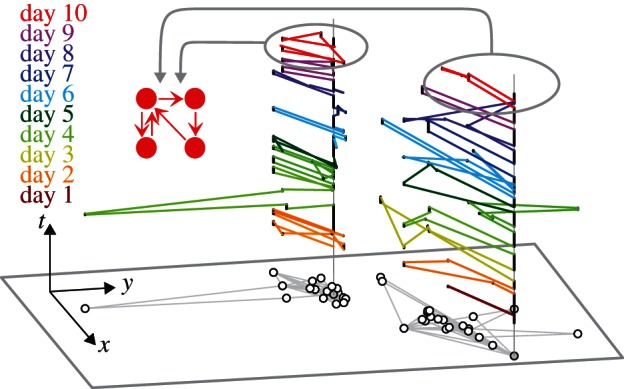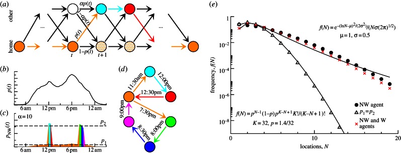By contrast, the daily average number of nodes is , and the average number of edges is . The left user prefers commuting to one place and visits the other locations during a single tour, whereas the right user prefers to visit the daily locations during a single tour. On the last day, both users visit not only four locations, but also share the same daily profile consisting of two tours with one and two destinations, respectively.

Figure 2.

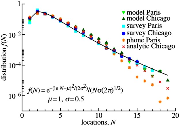
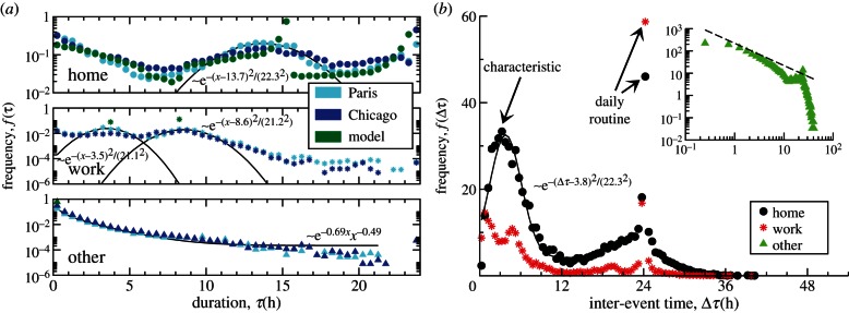
Daily human mobility patterns seem to follow a universal law. The daily number of visited locations can be approximated with a log-normal distribution with μ = 1 and σ = 0.5. The distributions extracted from activity and travel surveys as well as from mobile phone billing data show similar behaviour. Moreover, the distributions of our perturbation model (see §3 and figure 6 for details) generated both analytically and numerically have the same shape. The broad distribution shows that although most of the people visit less than five locations, a small fraction behave significantly differently because people report visits up to 17 different places within a day in our surveys. Note that due to the mobile phone data limitations, the tail of the corresponding distribution is below the other datasets.

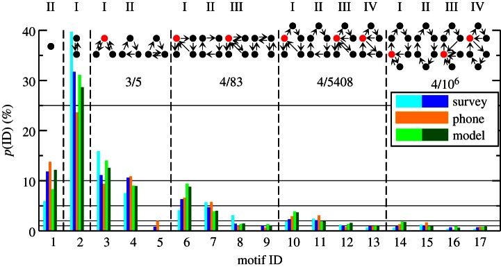
Figure 3.

Possible daily mobility patterns are limited, because up to 90% of the identified daily mobility networks can be described with only 17 different motifs. The probability p(ID) to find one of these 17 motifs in the surveys (cyan, Paris; blue, Chicago), the phone data (orange, Paris), and the model (light green, Paris; dark green, Chicago) is presented. The motifs are grouped according to their size separated by dashed lines. For each group, the fraction of observed over feasible motifs N_o/N_f is shown and the central nodes are highlighted. Most motifs can be classified by four rules: (I) motifs of size N consist of a tour with only one stop and another tour with N – 2 stops. (II) Motifs of size N consist of only a single tour with N stops. (III) Motifs of size N consist of two tours with one stop and another tour with N – 3 stops. (IV) Motifs of size N consist of a tour with two stops and another tour with N – 3 stops. Despite the fact that the number of workers is significantly different in both cities, the rank and the probability to find a specific motif exhibit similar behaviour.

Figure 4.

Daily human mobility patterns are stable over several months. The values, calculated by equation (2.3), show how more or less likely a motif is found during the observation period of six months under the condition that the individual has a given motif on another day. Positive values (yellow to red colours) indicate that these motifs are more likely than expected and negative values (cyan to blue colours) that these motifs are suppressed. The probability to find the same daily motif during another day is significantly larger compared with the randomized dataset. Additionally, active users, which visit more than four locations per day, seem to be active over time, whereas inactive users remain inactive. The emerging patterns of transitions between active motifs could be explained by the similarity of motifs. While transitions between motifs of group II are preferred, transitions between groups II and III are suppressed, because the number of tours is most different. As a guide to the eye, motifs with the same number of locations are marked with boxes.

Figure 5.

Fundamental differences between home/work and other locations. (a) The duration spent at either home or work is relatively flat distributed with peaks around characteristic time spans of 14 h at home as well as 3.5 and 8.6 h at work. By contrast, the time spent at other activities is broadly distributed. For a guide to the eye, Gaussian distributions are fitted around the characteristic durations for home/work locations and a power law with an exponential cut-off is fitted for other locations. Our model captures these main characteristics. (b) The frequency of observing an inter-event time τ between the beginning of two similar activities, if another location has been visited in between. For the home and work location, daily routines dominate the distribution with additional characteristic times. By contrast, the distribution for other locations exhibits a broad distribution dominated by short inter-event times with a suppressed daily routine. For a guide to the eye, the characteristic inter-event time between home location is approximated by a Gaussian distribution and in the inset a power law with exponent −1 is included.

Figure 6.

The introduced model is illustrated for a non-working agent. (a) The possible trajectories of an agent are shown. The agent starts the day at home and finishes it at home. At a given time t, depending on the actual location of the agent, the probability to be at home at time t + 1 is either 1 − p(t) or 1 − αp(t) with a parameter α and with probability p(t) and αp(t) the agent travels to another location. The filled circles and the coloured path is an exemplary trajectory. The time-dependent probabilities can be related to the circadian rhythm of activity, shown in (b). (c) The location-dependent probabilities for the exemplary agent with α = 10 are shown. The time-dependent probabilities can be approximated by only two values, p₁ and p₂ for being at home and being at another location. With this approximation, the model can be solved analytically. (d) The exemplary trajectory is converted into the corresponding motif with six locations and seven trips among them. (e) The daily number of visited locations obtained from the analytical model under three different conditions is shown. While the removal of workers does not change the tail of the log-normal distribution, α = 1 leads to a binomial distribution; thus periods of activities are key for the observed behaviour. Note that the absolute difference between analytical and numerical model is less than 0.01.

References

1. Anderson RM, May RM. 1992. Infectious diseases in humans. Oxford, UK: Oxford University Press
1. Lloyd AL, May RM. 2001. How viruses spread among computers and people. Science 292, 1316–131710.1126/science.1061076 (doi:10.1126/science.1061076) - DOI - DOI - PubMed
1. Hufnagel L, Brockmann D, Geisel T. 1992. Forecast and control of epidemics in a globalized world. Proc. Natl Acad. Sci. USA 101, 15124–1512910.1073/pnas.0308344101 (doi:10.1073/pnas.0308344101) - DOI - DOI - PMC - PubMed
1. Colizza V, Pastor-Satorras R, Vespignani A. 2007. Reaction–diffusion processes and metapopulation models in heterogeneous networks. Nat. Phys. 3, 276–28210.1038/nphys560 (doi:10.1038/nphys560) - DOI - DOI
1. Balcan D, Colizza V, Goncalves B, Hu H, Ramasco JJ, Vespignani A. 2009. Multiscale mobility networks and the spatial spreading of infectious diseases. Proc. Natl Acad. Sci. USA 106, 21 484–21 48910.1073/pnas.0906910106 (doi:10.1073/pnas.0906910106) - DOI - DOI - PMC - PubMed
Publication types
LinkOut - more resources