Synergies between intrinsic and synaptic plasticity based on information theoretic learning

Abstract

In experimental and theoretical neuroscience, synaptic plasticity has dominated the area of neural plasticity for a very long time. Recently, neuronal intrinsic plasticity (IP) has become a hot topic in this area. IP is sometimes thought to be an information-maximization mechanism. However, it is still unclear how IP affects the performance of artificial neural networks in supervised learning applications. From an information-theoretical perspective, the error-entropy minimization (MEE) algorithm has newly been proposed as an efficient training method. In this study, we propose a synergistic learning algorithm combining the MEE algorithm as the synaptic plasticity rule and an information-maximization algorithm as the intrinsic plasticity rule. We consider both feedforward and recurrent neural networks and study the interactions between intrinsic and synaptic plasticity. Simulations indicate that the intrinsic plasticity rule can improve the performance of artificial neural networks trained by the MEE algorithm.

Figure 1. Structure of the feedforward neural networks.

Figure 2. Structure of the recurrent neural networks.

Figure 3. Learning curves of the quadratic information potential by the FNN.

The dashed lines denote the learning curves of the MEE algorithm, and the solid lines denote the learning curves of the synergistic algorithm. (A) 300-epoch learning curves for the training data set “MG”. (B) 1000-epoch learning curves of “MG”. (C) 300-epoch learning curves for the training data set “SS”. (D) 1000-epoch learning curves of “SS”.

Figure 4. Learning curves of the mean square error by the FNN.

The dashed lines denote the learning curves of the MEE algorithm, and the solid lines denote the learning curves of the synergistic algorithm. (A) 300-epoch learning curves for the training data set “MG”. (B) 1000-epoch learning curves of “MG”. (C) 300-epoch learning curves for the training data set “SS”. (D) 1000-epoch learning curves of “SS”.

Figure 5. Decomposition of the FNN.

(A) The input layer and the hidden layer of the FNN. (B) The output layer of the FNN.

Figure 6. Input and output distributions for neurons in the hidden layer of the FNN.

Input and output distributions for the five hidden neurons with the training data set “MG” are displayed. (A) Initial input distributions for the five hidden neurons. (B) Input distributions after 1000-epoch training for the two algorithms. (C) Initial output distributions for the five hidden neurons. (D) Output distributions after 1000-epoch training for the two algorithms. In (B) and (D), the dash lines denote the distributions obtained by the MEE algorithm, and the solid lines denote the distributions obtained by the synergistic algorithm.

Figure 7. Input distributions for the output neuron and error distributions of the FNN.

Input distributions for the single output neuron and error distributions with the training data set “MG” are presented. (A) Initial input distribution. (B) Input distributions after 1000-epoch training for the two algorithms. (C) Initial error distribution. (D) Error distributions after 1000-epoch training for the two algorithms. In (B) and (D), the dash lines denote the distributions obtained by the MEE algorithm, and the solid lines denote the distributions obtained by the synergistic algorithm.

Figure 8. Evolution of the parameters of the activation functions in the FNN.

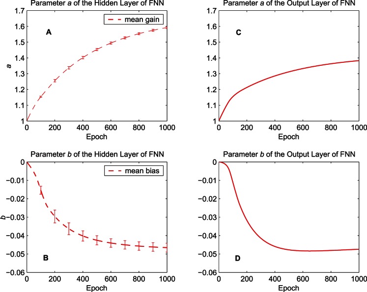
The training data set “MG” is used. (A) Mean of the gain parameter of the five hidden neurons. (B) Mean of the bias parameter of the five hidden neurons. (C) The gain parameter of the output neuron. (D) The bias parameter of the output neuron.

Figure 9. Learning curves of the FNN with different IP learning rates.

The training data set “MG” is used. The initial IP learning rates , , , and (no IP) are used for comparison. Learning curves of the quadratic information potential: (A) 300 epochs. (B) 1000 epochs. Learning curves of the mean square error: (C) 300 epochs. (D) 1000 epochs.

Figure 10. Relation between the training result and the number of hidden neurons of the FNN.

Training results after 1000-epoch training for the case of the training data set “MG” are presented. The circle markers denote the results obtained by the MEE algorithm, and the cross markers denote the results obtained by the synergistic algorithm. (A) Results of the quadratic information potential. (B) Results of the mean square error.

Figure 11. Learning curves of the quadratic information potential by the RNN.

The dashed lines denote the learning curves of the MEE algorithm, and the solid lines denote the learning curves of the synergistic algorithm. (A) 300-epoch learning curves for the training data set “MG”. (B) 1000-epoch learning curves of “MG”. (C) 300-epoch learning curves for the training data set “SS”. (D) 1000-epoch learning curves of “SS”.

Figure 12. Learning curves of the mean square error by the RNN.

The dashed lines denote the learning curves of the MEE algorithm, and the solid lines denote the learning curves of the synergistic algorithm. (A) 300-epoch learning curves for the training data set “MG”. (B) 1000-epoch learning curves of “MG”. (C) 300-epoch learning curves for the training data set “SS”. (D) 1000-epoch learning curves of “SS”.

Figure 13. Input, output and error distributions for neurons of the RNN.

The training data set “MG” is used. Neuron 1 (output neuron): (A) Initial input distribution. (B) Input distributions after 1000-epoch training for the two algorithms. (C) Initial error distribution. (D) Error distributions after 1000-epoch training for the two algorithms. Neuron 2: (E) Initial input distribution. (F) Input distributions after 1000-epoch training for the two algorithms. (G) Initial output distribution. (H) Output distributions after 1000-epoch training for the two algorithms. In (B), (D), (F), and (H), the dash lines denote the distributions obtained by the MEE algorithm, and the solid lines denote the distributions obtained by the synergistic algorithm.

Figure 14. Evolution of the parameters of the activation functions in the RNN.

The training data set “MG” is used. (A) The gain parameter . (B) The bias parameter .

Figure 15. Learning curves by the RNN with different IP learning rates.

The training data set “MG” is used. The initial IP learning rates , , , and (no IP) are used for comparison. Learning curves of the quadratic information potential: (A) 300 epochs. (B) 1000 epochs. Learning curves of the mean square error: (C) 300 epochs. (D) 1000 epochs.

Figure 16. Relation between the training result and the number of neurons of the RNN.

Training results after 1000-epoch training for the case of the training data set “MG” are presented. The circle markers denote the results obtained by the MEE algorithm, and the cross markers denote the results obtained by the synergistic algorithm. (A) Results of the quadratic information potential. (B) Results of the mean square error.

References

1. Principe JC (2010) Information theoretic learning: Renyi’s entropy and kernel perspectives. New York, Dordrecht, Heidelberg, London: Springer.
1. Marder E, Abbott LF, Turrigiano GG, Liu Z, Golowasch J (1996) Memory from the dynamics of intrinsic membrane currents. Proc Natl Acad Sci USA 93: 13481–13486. - PMC - PubMed
1. Desai NS, Rutherford LC, Turrigiano GG (1999) Plasticity in the intrinsic excitability of cortical pyramidal neurons. Nat Neurosci 2: 515–520. - PubMed
1. Zhang W, Linden DJ (2003) The other side of the engram: Experience-driven changes in neuronal intrinsic excitability. Nat Rev Neurosci 4: 885–900. - PubMed
1. Daoudal G, Debanne D (2003) Long-term plasticity of intrinsic excitability: Learning rules and mechanisms. Learn Mem 10: 456–465. - PubMed
Publication types
LinkOut - more resources