Visually driven chaining of elementary swim patterns into a goal-directed motor sequence: a virtual reality study of zebrafish prey capture

Abstract

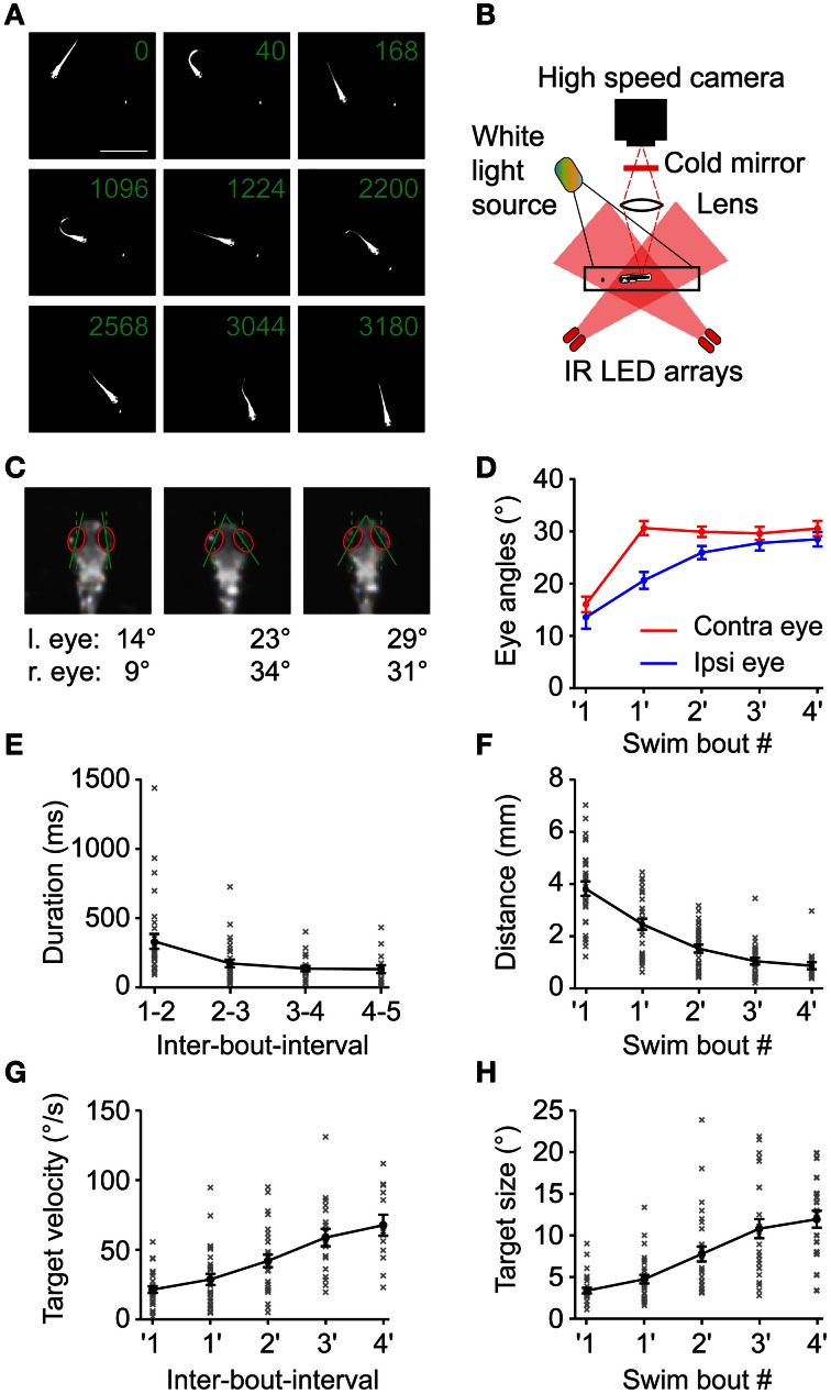
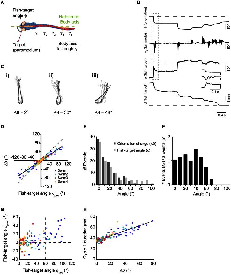
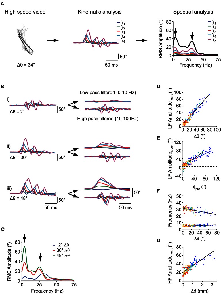
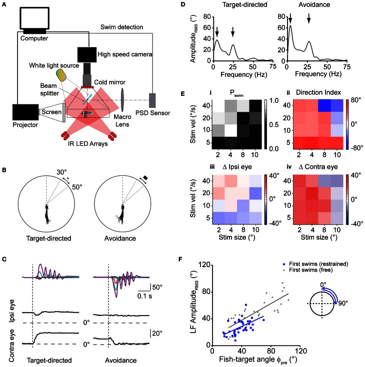
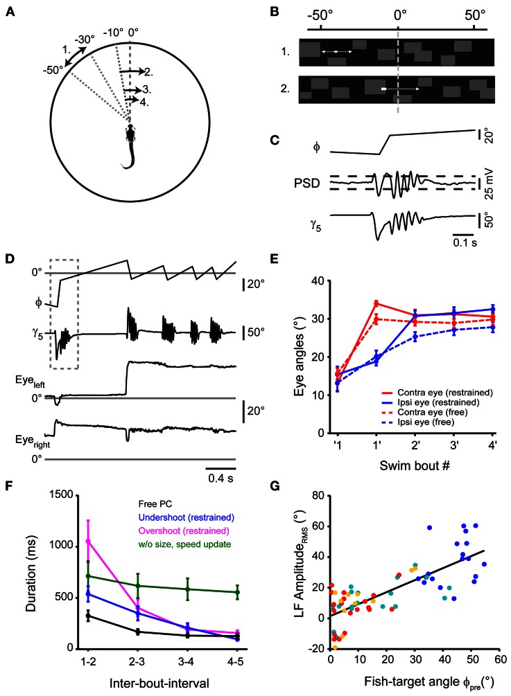
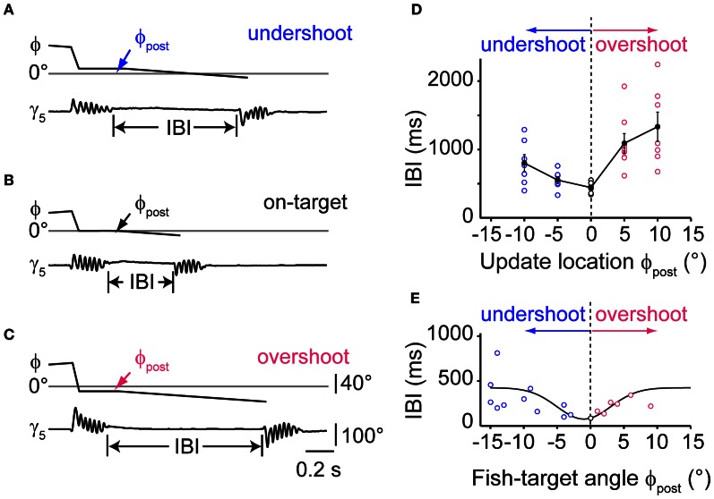
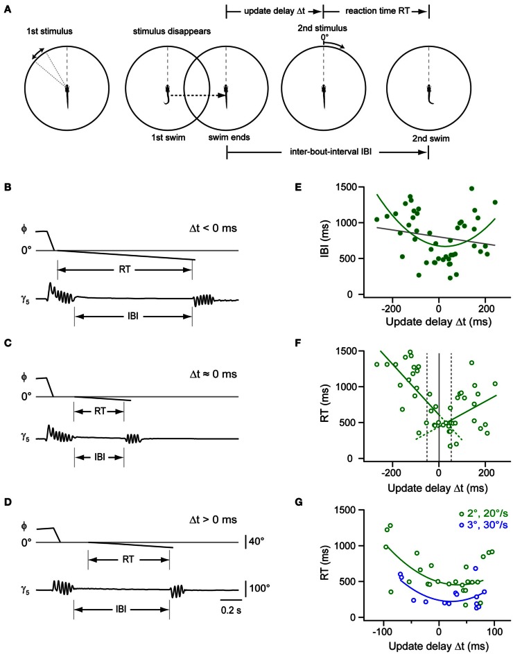
Prey capture behavior critically depends on rapid processing of sensory input in order to track, approach, and catch the target. When using vision, the nervous system faces the problem of extracting relevant information from a continuous stream of input in order to detect and categorize visible objects as potential prey and to select appropriate motor patterns for approach. For prey capture, many vertebrates exhibit intermittent locomotion, in which discrete motor patterns are chained into a sequence, interrupted by short periods of rest. Here, using high-speed recordings of full-length prey capture sequences performed by freely swimming zebrafish larvae in the presence of a single paramecium, we provide a detailed kinematic analysis of first and subsequent swim bouts during prey capture. Using Fourier analysis, we show that individual swim bouts represent an elementary motor pattern. Changes in orientation are directed toward the target on a graded scale and are implemented by an asymmetric tail bend component superimposed on this basic motor pattern. To further investigate the role of visual feedback on the efficiency and speed of this complex behavior, we developed a closed-loop virtual reality setup in which minimally restrained larvae recapitulated interconnected swim patterns closely resembling those observed during prey capture in freely moving fish. Systematic variation of stimulus properties showed that prey capture is initiated within a narrow range of stimulus size and velocity. Furthermore, variations in the delay and location of swim triggered visual feedback showed that the reaction time of secondary and later swims is shorter for stimuli that appear within a narrow spatio-temporal window following a swim. This suggests that the larva may generate an expectation of stimulus position, which enables accelerated motor sequencing if the expectation is met by appropriate visual feedback.

Keywords: double-step saccade; goal-directed behavior; intermittent locomotion; motor sequence; prey capture; saccadic suppression; virtual reality; zebrafish.

Figure 1

Swim sequences during prey capture behavior. (A) Selected frames of a 6 dpf larva performing a prey capture sequence recorded at 250 frames/s showing swim and rest episodes. Same field of view for all 9 frames (scale bar: 4 mm). Only one paramecium present (elongated white object, highlighted by local contrast enhancement). Numbers in each frame indicate time in milliseconds. Frames 2, 4, 6, and 8 show the 1st, 2nd, 4th and the capture swim in the sequence, respectively. (B) Experimental setup to record high speed movies of freely moving larva capturing prey. (C) Ipsilateral and contralateral eye angle measurements before 1st, after 1st and after 2nd swim. Magnified view of larval head, rotated to an upright position for clarity. Red ellipses: outline of the eyes, solid lines: major axis of ellipses; dashed lines: fish heading direction. (D) Ipsilateral and contralateral eye angles during the prey capture sequence (mean ± sem; n = 30 sequences). Note: eyes are specified as ipsilateral or contralateral based on the location of the prey target before the first swim of the sequence. This assignment was maintained for eye angle measurements made throughout the sequence irrespective of the location of the target in successive swims. (E) The interval between two successive swim bouts (IBI) decreased monotonically as the sequence progressed (n = 30 sequences). (F) Distance between the larva and the prey decreased monotonically with each swim from 3.8 ± 0.27 mm before first swim to 0.89 ± 0.13 mm after 4th swim. (G) Angular velocity of the prey measured between two swims increased monotonically from 21.1°/s ± 2.3°/s before first swim to 67°/s ± 7.5°/s after 4th swim. (H) Angular size of the prey increased from 3.2° ± 0.3° before first swim to 11.9° ± 1° after 4th swim. In (D), (F), (G), and (H), ′1 indicates measurements immediately before the first swim of a sequence, while 1′ indicates measurements immediately after the first swim and so on.

Figure 2

Single swims cover a large angular range, controlled by target position. (A) Illustration depicting automated image processing and parameter extraction from an individual frame. Colored contour lines represent distance map of the fish body. Six segments were used to fit the midline (Solid orange line: head segment; solid red lines: the tail split into five equidistant segments). Broken green line represents body axis with reference to which the deviations of the tail segments (γ₁,…, γ₅) were measured. (B) Time course of analyzed parameters for the sequence shown in Figure 1A on a frame-by-frame basis. Inset shows a blow up of the first swim bout of the sequence (dashed box). (C) Three examples (i,ii, and iii) of swims associated with change in orientation of 2, 30, and 48°, respectively. Every 10th frame (frame rate: 500/s) of the fish contour is overlaid. Light to dark contours indicate the progress of the swim bout from beginning to end. (D) Scatter plot of the change in body orientation (Δθ) generated by a swim bout vs. fish-target angle (ϕ_pre) preceding the swim. Broken line: unity line; Solid line: straight line fit. (E) Histogram of fish-target angle (ϕ_pre) and change in orientation (Δθ) from the data shown in (D). Data were grouped into 10°-bins (1st bin contains angles from −5 to 5°, 2nd bin contains angles from −5 to −15° and from 5 to 15°, and so on). (F) Histogram of the orientation change (Δθ), normalized to the occurrence of fish-target angles (ϕ_pre) for the data shown in (D). Bin width as in (E). (G) Scatter plot of fish-target angle after each swim (ϕ_post) vs. fish-target angle before the swim (ϕ_pre). Data points with negative fish-target angles (corresponding to prey on left side) were point-reflected about the origin. (H) Scatter plot of duration of first cycle in a swim bout vs. the resulting change in orientation. Data points with negative changes in orientation (corresponding to swims toward the left) were mirror-reflected about the y-axis. In (D), (G), and (H), data points are color-coded to show the 1st, 2nd, 3rd, and 4th swims during a sequence.

Figure 3

Spectral analysis of individual swim bouts of the freely moving larva during prey capture. (A) Schematic representation of spectral analysis of single swim bouts. Left: fish contours of a swim bout. Center: time course of tail angles (γ₁, …, γ₅) obtained from automated tail angle measurement. Right: Fourier transform of each of the tail angle traces (γ₁, …, γ₅) results in individual RMS amplitude spectra shown in the corresponding color. Sum of these individual spectra is shown as bold black curve. Note two peaks in the spectra (arrows). (B) Left: time course of tail angles (γ₁, …, γ₅) for the three swim examples shown in Figure 2C. Right: time course of tail angles after low- and high-band-pass filtering. (C) Summed RMS amplitude spectra for the three swim bouts shown in (B). Note two peaks in the amplitude spectra (arrows) at frequencies similar to those in (A, right panel). The peak at lower frequencies (~4 Hz) scales with change in orientation (Δθ). (D) Scatter plot of the low-frequency (LF) peak amplitude from spectral analysis vs. change in orientation (Δθ). Colors indicate swim bout number (as in Figure 2). (E) Scatter plot of the low-frequency peak amplitude from spectral analysis vs. fish-target angle (ϕ_pre) preceding the swim. Solid lines: straight line fits to the data pairs from first swims (blue) and subsequent swims (black) during a sequence. Note shallower slope for first swims. Same color code as in (D). (F) Scatter plot of the location of the high frequency peak (crosses) and low frequency peak (circles) vs. the change in orientation after each swim (Δθ). Lines are straight line fits to the data. Same color code as in (D). (G) Scatter plot of high-frequency (HF) peak amplitude vs. change in fish-target distance (Δd) after the swim bout. Same color code as in (D).

Figure 4

Virtual prey-like stimuli evoke swims similar to motor patterns during prey capture. (A) Illustration depicting the setup used to record swim bouts in response to visual stimuli presented to minimally restrained larvae. A position-sensitive device (PSD, right) is used to detect swims and update the visual stimulus at high speed. (B) Left: swim bout toward a rectangular stimulus (width × height: 2 × 1°), moving at 20°/s peripherally between 30 and 50°. Right: swim bout toward the opposite direction of a rectangular stimulus (8 × 4°) moving at 40°/s. Every 10th frame of the high speed movies during the swim bout is overlaid. Angular dimensions drawn to scale. Fish and chamber dimensions not drawn to scale. (C) Time course of tail angles and ipsilateral and contralateral eye angles for the examples shown in (B) obtained using automated image analysis. Same color code as in Figure 3A. Note: high spatial resolution during imaging of restrained larvae allowed automated eye angle analysis. (D) Summed RMS amplitude spectra obtained from traces in (C) for the target-directed (left) and avoidance swim bout (right). Note two peaks in the spectra (arrows), similar to spectra measured in freely moving larvae during prey capture. (E) Summary of motor output in response to 16 different combinations of size and velocity of a moving stimulus. Panel (i): probability of observing a swim bout during a 60 s interval of stimulus presentation. Panel (ii): direction index calculated from LF peaks in the amplitude spectrum, showing target-directed, and avoidance turns (red and blue squares, respectively). Panel (iii): change in position of ipsilateral eye. Positive values indicate rotation to more nasal position. Panel (iv): same as panel (iii), but for contralateral eye. Positive values indicate rotation to more nasal position. In panels (ii–iv), colors indicate mean values (n = 6–12 trials for each stimulus parameter pair). Note: for each panel, the value of the target size denotes the width of the stimulus and width:height ratio is always 2:1. (F) Scatter plot of the LF peak amplitude_rms from spectral analysis vs. fish-target angle (ϕ_pre) immediately preceding the swim. A trial consisted of the stimulus moving from center to periphery (rostro-caudal) or periphery to center (caudo-rostral), where it disappeared. Stimulus size and velocity 2° and 20°/s, respectively. Blue solid line: straight line fit. Also shown are data pairs (LF peak amplitude_rms; ϕ_pre) and straight line fit from first swims in freely moving larvae (gray symbols; same data as in Figure 3E).

Figure 5

Virtual prey capture behavior in a closed-loop system. (A) Illustration depicting the stimulus update paradigm used to evoke prey capture-like swim sequences in minimally restrained larvae. Numbers indicate order of appearance of moving stimulus, arrows indicate direction. Here, following detection of a swim, the stimulus was translated to −10°, from where it moved across the midline into the contralateral visual hemifield. Target size and velocity were increased following each swim, emulating an approach of the larva toward the target. This is illustrated by reducing the distance of arrows in the diagram. (B) Representation of the stimulus from the perspective of the larva. Initially, a rectangular target moves in the periphery against a background of low spatial frequency content (upper panel). At the onset of a swim bout, target and background translate smoothly toward the visual field center (within ±10°, update velocity ~400°/s), emulating a change in orientation of the fish toward the target. Subsequently, the target continues to move against the background (lower panel). (C) Detection of swim bouts. Bottom: time course of caudal tail angle γ₅, during a target-directed swim bout. Center: time course of PSD voltage during the swim. Top: fish-target angle (ϕ) before, during, and after the swim bout. Target and background rotation were triggered in real-time by threshold-crossing of the PSD signal (indicated by dashed horizontal lines). (D) A swim sequence resembling prey capture sequences in freely moving larvae, recorded in a minimally restrained larva. Top: time course of fish-target angle ϕ. Second from top: caudal tail angle γ₅. Dashed box indicates temporal window shown in (C) on an expanded scale. Bottom two traces: left and right eye angle traces. (E) Comparison of ipsilateral eye angles (15.4 ± 2.1° before first swim; 32.5 ± 1.1° after 4th swim) and contralateral eye angles (13.1 ± 2.2° before first swim; 30.6 ± 1.3° after 4th swim) during sequences in restrained larvae (solid line; n = 19 sequences) to eye angles in freely moving larvae (broken line; n = 30 sequences). (F) Comparison of inter-bout-intervals (IBIs) for different stimulus conditions. Black line: IBIs during prey capture sequences in freely moving larvae (n = 30 sequences). Blue line: IBIs during sequences of restrained larvae, where target is translated to −10° during the first swim, representing undershoot (n = 11 sequences). Magenta line: IBIs during sequences of restrained larvae, where target is translated to +10° during the first swim, representing overshoot (n = 8 sequences). Green line: IBIs during sequences of restrained larvae, where target is translated to −10° during the first swim, representing undershoot, but without increases in stimulus size and velocity throughout the sequence (n = 6 sequences). (G) Scatter plot of the LF peak amplitude from spectral analysis vs. fish-target angle (ϕ_pre) immediately preceding the swim (n = 19 sequences). Same color code as in Figure 2.

Figure 6

Timing of sequenced swim bouts depends on updated stimulus location. (A) Time course of fish-target angle ϕ and caudal tail angle γ₅ during a pair of swim bouts evoked by a moving target in a restrained larva. First swim was directed toward a stimulus moving in the periphery (35–55°). Onset of the first swim triggered a translation of stimulus/background stopping short 10° from the midline, simulating an undershoot in turning. The end of the first swim triggered stimulus motion at constant velocity toward the contralateral hemifield, evoking a second, target-directed swim. Inter-bout-interval (IBI) indicated by vertical lines. (B) Same as in panel (A), but with the stimulus/background translated to the center of the visual field (0°) during the first swim, simulating exact alignment of the larva with the location of prey (“on-target”). Note that the IBI is considerably shorter. (C) Same as in panel (A), but with the stimulus/background translated beyond the center of the visual field by 10° during the first swim, simulating an overshoot in turning. (D) Dependence of IBIs on the update location of the stimulus during the first swim bout. Trials with initial stimulus position on the left or right side were interspersed and pooled. Negative values of update location represent an undershoot; positive values an overshoot during the first swim. Data from n = 6 fish. (E) Data from recordings of freely moving larvae performing prey capture sequences. Scatter plot of IBIs between first and second swim bout in which the fish-target angle ϕ_post (measured at the end of the first swim) varied between ±15°. Negative values correspond to an undershoot, positive values to an overshoot in turning. Note the minimum in IBIs for small turning error near ϕ_post = 0°. Solid line is a Gaussian fit curve.

Figure 7

Impact of stimulus timing on inter-bout-intervals and reaction times in a two-step stimulus paradigm. (A) Schematic of a two-step stimulus paradigm with variable delay. First stimulus is a target moving in the periphery (35–55°; left panel), which eventually triggers a target-directed swim (second panel). Stimulus and background translate to center (0°), and the stimulus disappears. After a variable delay, the target reappears at the center and moves toward the periphery at constant size and speed (2°; 20°/s; 3rd panel), until the larva performs a second directed swim, which ends the trial (right panel). Update delays (Δt) and inter-bout-intervals (IBI) are measured relative to the end of the first swim, reaction time (RT) is measured from onset of second stimulus. (B) Time course of fish-target angle ϕ and caudal tail angle γ₅ during paired swim bouts evoked by the two-step stimulus paradigm. The second stimulus appeared before the end of the first swim, corresponding to a Δt < 0 ms. Note long IBI. (C) Same as in (B), but with second stimulus appearing near end of first swim (Δt ≈0 ms). Note short IBI. (D) Same as in (B), but with second stimulus appearing after end of first swim (Δt > 0 ms). Note longer IBI. Scale bars apply to panel (B–D). (E) Scatter plot of IBIs vs. update delay (Δt). Gray line: straight line fit (r_Pearson = 0.18). Green curve: second order polynomial fit to the data (r = 0.46). Note minimum near Δt ≈ 0 ms (n = 47 trials from 13 fish). (F) Scatter plot of reaction times (RT) vs. update delays (Δt). Green lines: straight line fits to data points with negative and positive update delays (Δt), respectively (n = 47 trials from 13 fish). Broken gray lines represent three different delay groups i.e., Δt < -50 ms, -50 ms < Δt < 50ms, and Δt > 50 ms. (G) Scatter plot of RT values vs. update delays (Δt) on an expanded time scale (–100 to 100 ms). Reaction times are shorter when the second stimulus is larger and faster (3°; 30°/s; n = 14 trials from 5 fish; blue symbols) than under control conditions [2°; 20°/s; green symbols, same as in panel (F)]. Blue and green curves are second order polynomial fits to data points measured under the two conditions, respectively.

References

1. Ahrens M. B., Li J. M., Orger M. B., Robson D. N., Schier A. F., Engert F., et al. (2012). Brain-wide neuronal dynamics during motor adaptation in zebrafish. Nature 485, 471–477 10.1038/nature11057 - DOI - PMC - PubMed
1. Avery R., Mueller C., Smith J., Bond D. (1987). The movement patterns of lacertid lizards: speed, gait and pauses in Lacerta vivipara. J. Zool. 211, 47–63
1. Bianco I. H., Kampff A. R., Engert F. (2011). Prey capture behavior evoked by simple visual stimuli in larval zebrafish. Front. Syst. Neurosci. 5:101 10.3389/fnsys.2011.00101 - DOI - PMC - PubMed
1. Bizzi E., Tresch M. C., Saltiel P., d'Avella A. (2000). New perspectives on spinal motor systems. Nat. Rev. Neurosci. 1, 101–108 10.1038/35039000 - DOI - PubMed
1. Boeddeker N., Egelhaaf M. (2005). A single control system for smooth and saccade-like pursuit in blowflies. J. Exp. Biol. 208, 1563–1572 10.1242/jeb.01558 - DOI - PubMed
Publication types
LinkOut - more resources