Frequency response areas in the inferior colliculus: nonlinearity and binaural interaction

Abstract

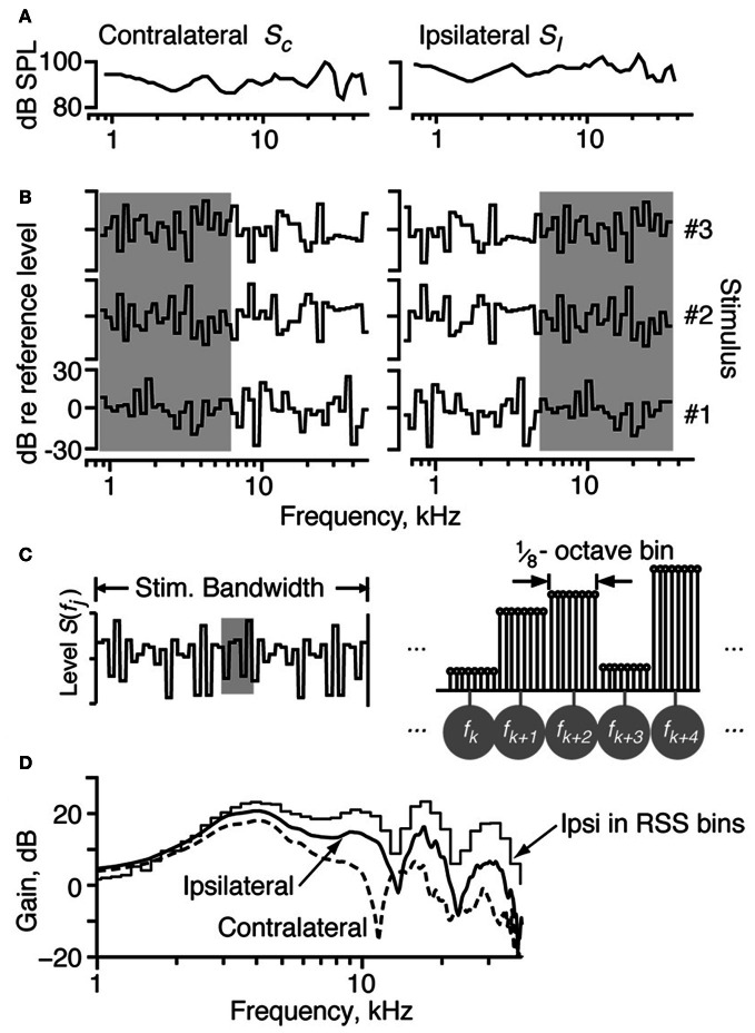
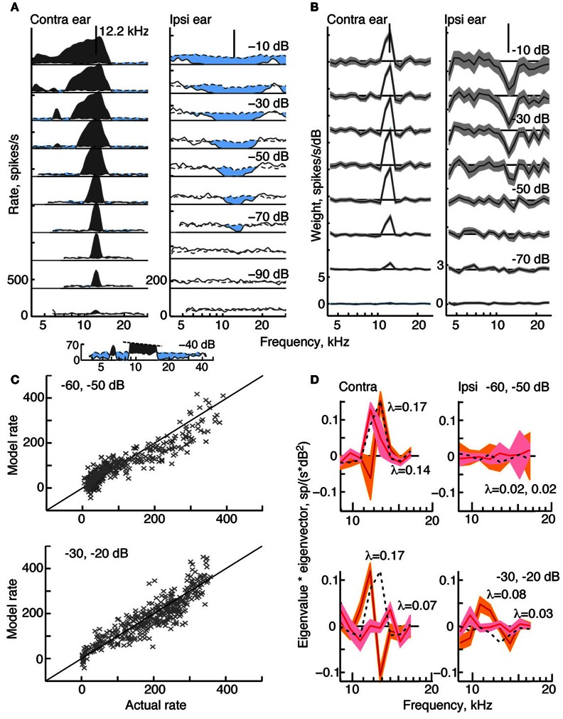
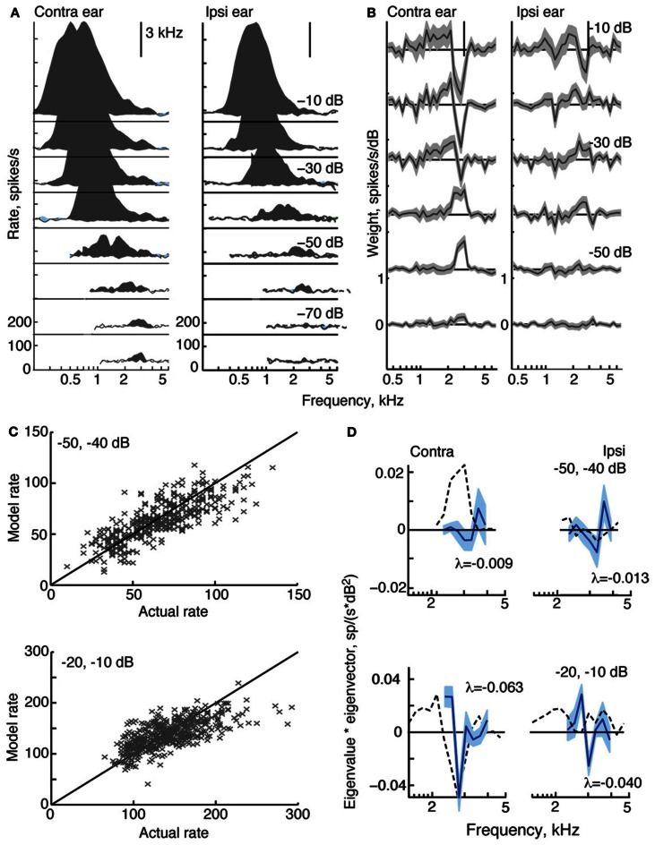
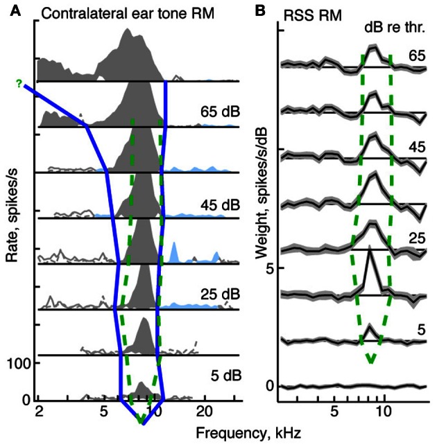
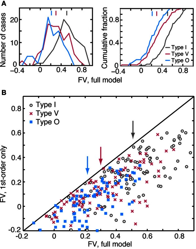
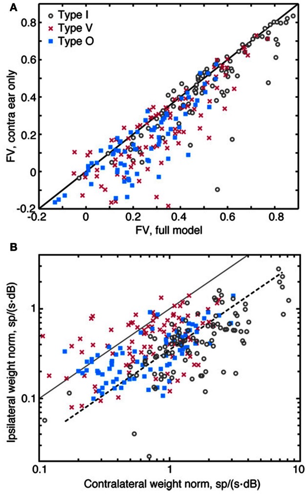
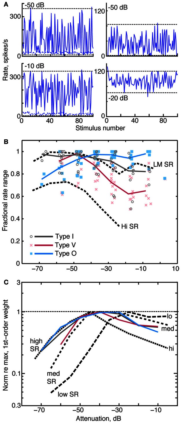
The tuning, binaural properties, and encoding characteristics of neurons in the central nucleus of the inferior colliculus (CNIC) were investigated to shed light on nonlinearities in the responses of these neurons. Results were analyzed for three types of neurons (I, O, and V) in the CNIC of decerebrate cats. Rate responses to binaural stimuli were characterized using a 1st- plus 2nd-order spectral integration model. Parameters of the model were derived using broadband stimuli with random spectral shapes (RSS). This method revealed four characteristics of CNIC neurons: (1) Tuning curves derived from broadband stimuli have fixed (i. e., level tolerant) bandwidths across a 50-60 dB range of sound levels; (2) 1st-order contralateral weights (particularly for type I and O neurons) were usually larger in magnitude than corresponding ipsilateral weights; (3) contralateral weights were more important than ipsilateral weights when using the model to predict responses to untrained noise stimuli; and (4) 2nd-order weight functions demonstrate frequency selectivity different from that of 1st-order weight functions. Furthermore, while the inclusion of 2nd-order terms in the model usually improved response predictions related to untrained RSS stimuli, they had limited impact on predictions related to other forms of filtered broadband noise [e. g., virtual-space stimuli (VS)]. The accuracy of the predictions varied considerably by response type. Predictions were most accurate for I neurons, and less accurate for O and V neurons, except at the lowest stimulus levels. These differences in prediction performance support the idea that type I, O, and V neurons encode different aspects of the stimulus: while type I neurons are most capable of producing linear representations of spectral shape, type O and V neurons may encode spectral features or temporal stimulus properties in a manner not easily explained with the low-order model. Supported by NIH grant DC00115.

Keywords: binaural; dynamic range; inferior colliculus; level tolerant; model; nonlinearity; random spectral shape; tuning.

Figure 1

The properties of the RSS stimuli. (A) The acoustic calibration of the two ears in one animal, showing the sound pressure level as a function of frequency at 0 dB attenuation. These were determined using a calibrated probe tube placed within 2 mm of the eardrum. The spectra of sounds were modified by filtering with these transfer functions. (B) Spectra of three example RSS stimuli, out of the set of 200, shown as the dB spectrum level vs. log frequency. The sound levels of individual frequency bins (of width 1/8 octave) are symmetrically distributed around a mean value of 0 dB, with SD 12 dB. The reference 0-dB sound level is varied with an attenuator, usually over a 50–70 dB range. Note that the spectra presented to the ipsilateral ear are frequency-shifted versions of the spectra presented to the contralateral ear (e.g., compare gray areas). (C) Spectral shape of the RSS stimuli in more detail. Each frequency bin consists of 8 tones, logarithmically spaced at 1/64 octave. Individual tones are shown in the line spectrogram at right, which corresponds to the shaded region of the stimulus spectrum at left. The eight tones in each bin (1/8 octave wide) have equal sound level. Frequencies of the bin centers are indicated by the symbols in gray circles. (D) Spectra of white noise filtered with two cat HRTFs. The ipsilateral and contralateral HRTFs approximate the spectral shapes in the ipsilateral and contralateral ears of a broadband noise stimulus played at 15° azimuth, 30° elevation. The stepped-function (“Ipsi in RSS bins”) shows the stimulus energy for the ipsilateral spectrum in bins corresponding to the RSS stimuli at a sampling rate of 100 kHz.

Figure 2

Response characteristics for a type I neuron, BF 12.2 kHz. (A) Tone response maps showing rate responses to 200-ms tone bursts, plotted against the tone frequency at a fixed attenuation. Rates were computed from single tone presentations and smoothed (5-bin triangular filter) for display. Attenuations are shown at right. Zero dB attenuation was 94 dB SPL at the neuron's BF. Response maps were created by presenting tones in the contralateral ear only (left) and ipsilateral ear only (right). Discharge rates across the duration of the tone are shown by solid lines. Spontaneous rates are shown by dashed lines. The horizontal solid straight line indicates 0 spikes/s, and the rate scale is given at bottom left (different in the two ears). Excitatory responses are colored gray and inhibitory responses are light blue. The vertical lines at the top of the plots show the BF in the contralateral ear (12.2 kHz). (B) Weight functions estimated from responses to binaural RSS stimuli presented across a range of attenuations. First-order weights (w_C and w_I in Equation 1) are plotted on the same frequency axis as in (A). Weight estimates are shown as black lines, and gray regions indicate ±1 SEM. Contralateral and ipsilateral weight functions were derived from the same 200 responses to the binaural stimulus set. Note that the weight scales on the ordinate differ. (C) Rates predicted by the model (ordinate) vs. experimental rates (abscissa) in leave-one-out model testing. For each plot, data for two attenuations (indicated in the legend) were combined for the leave-one-out procedure. (D) Second-order effective filters (i. e., eigenvectors of M_C and M_I in Equation 3) for the same two fits shown in (C). Eigenvectors multiplied by their corresponding eigenvalue are plotted against frequency. The 1st-order weights, scaled to the same maximum value in each plot, are shown as black dotted lines. Only eigenvectors with the two largest positive eigenvalues λ are shown (largest λ, orange; second-largest λ, pink). The colored regions indicate ±1 SEM. The negative eigenvalues are smaller than the positive eigenvalues (<0.03, top case; <0.1, bottom case) and the corresponding eigenvectors are noisy (not shown).

Figure 3

Response characteristics for a type O neuron, BF 11.4 kHz. (A,B) Tone response maps and RSS weight functions, plotted as in Figure 2. Note the large inhibitory area centered on BF in the contralateral and ipsilateral tone response maps. Also note the difference in shape of the tone and weight-function maps. 0 dB attenuation is 98 dB SPL at the BF of the neuron. (C) Prediction performance as in Figure 2. fv-values are 0.54 for the stimuli at −60/−50 dB, and 0.51 at −20/−10 dB. (D) 2nd-order weight functions with the largest eigenvalues, given in the legends. Weights with positive eigenvalues are shown in red, and weights with negative eigenvalues are shown in blue.

Figure 4

Response characteristics for a type V neuron, BF = 3 kHz. (A) Response maps, plotted as in Figure 2. Zero dB attenuation was 98 (contra) and 95 (ipsi) dB SPL at the BF of the neuron. (B) At high sound levels, 1st-order weight functions suggest a substantial inhibitory area around BF–a pattern consistent with the weak responses to tones near BF in (A). (C) Prediction performance as in Figure 2. fv-values are 0.61 for the stimuli at −50/−40 dB, and 0.41 at −20/−10 dB. (D) 2nd-order weights with the largest negative eigenvalues, given in the legends.

Figure 5

Derivation of tuning curves from response maps for a type I neuron (BF = 8.3 kHz). (A) Tone response map for the contralateral ear. The blue curve shows the tuning curve edges for the tone response map, derived as described in the text. The green dashed curve in both (A) and (B) shows the edges of the tuning curve for the weight-function map. (B) Weight-function map for the same neuron. The dB scale in both parts is dB re threshold for BF tones (A) or RSS stimuli (B). The tuning curve near the BF tip is not well specified by the response maps. For the tone response maps, the threshold at BF is determined from a rate-level function; for the weight-function maps, the threshold is set halfway between levels that do and do not produce weights that are significantly different than zero.

Figure 6

Level tolerance of the edges of tone and weight-function response maps for populations of type I (A), O (B), and V (C) neurons. Frequency edges computed as in Figure 5 are shown for contralateral stimuli only. Lower-(left) and upper-(right) frequency edges derived from tone response maps (blue lines) are overlaid on those derived from weight-function maps (dashed green lines) at equivalent sound levels, in dB re threshold. The point at BF is not included. For each neuron, lower (or upper) edge frequencies are plotted relative to the geometric mean across levels of the lower (or upper) edge frequencies of the weight-function maps. Slopes of lower frequency edges of tone maps differ significantly from those observed in weight-function maps (type I: P = 0.1; type V: P < 0.01; signed rank sum comparisons of slopes of best-fit lines). Upper-frequency edges do not differ. Tone maps were not analyzed for type O neurons (see text). The red curves in (B) show mean weight-function edges for auditory nerve fibers [ANF; data from Figure 5 of Young and Calhoun (2005)]. Here, frequencies are normalized by the average frequency edge at the lowest two sound levels. As sound level increases, the slopes of lower-frequency edges of CNIC weight-functions differ from those observed in ANF. Specifically, slopes suggest a relative narrowing in type I and type O data (P = 0.02), and relative widening in type V neurons (P = 0.07). For all weight-function types, upper frequency edges are not significantly different from those seen in ANFs. All Ps are Bonferroni corrected.

Figure 7

Quality of the model predictions as measured by fv in leave-one-out cross validation tests. Each plot contains an aggregation of prediction data obtained at different sound levels. A neuron is usually represented multiple times, once at each sound level and also at pairs of adjacent sound levels. (A) Distribution (left) and cumulative distribution (right) of fv-values for the three response types. Vertical lines at the top of the plots show median fv-values. Differences in the distributions across the neuron types are statistically significant (rank sum test with Bonferroni correction; I vs. V and I vs. O, P << 0.001; V vs. O, P < 0.02). (B) Comparison of the best prediction quality (fv) for a full binaural model containing all 2nd-order terms (abscissa) and a model containing only 1st-order terms (ordinate). Ten data points with ordinate values <−0.2 are not shown, but are included in the statistics. Vertical arrows indicate median fv-values for each of the neuron types.

Figure 8

Prediction quality for RSS and HRTF stimuli by sound level. (A) Quality of RSS response predictions (fv) plotted against the sound level of the stimulus. Light colored symbols connected by lines show data obtained from one neuron. Heavy colored lines show median fv-values for the 3 neuron types. For clarity in plotting, 1 dB was added to the attenuations for V neurons, and 2 dB was added to the attenuations for O neurons. (B) Predicted rate responses to HRTF-filtered noise (VS stimuli), computed using weight-function models derived at the same overall sound level (−40 dB). Predictions for a type I (left) and a type O (right) neuron were computed using the difference method (see text). Actual rates are shown in green and predicted rates are shown in blue. The goodness of fit for these predictions are as follows: Type I (left): R² = 0.82, fv = 0.7; type O (right): R² = 0.39, fv = 0. (C) Median R² for the three neuron types. Solid lines indicate median R²-values obtained when the full model was used to predict responses to VS stimuli; dashed lines indicate median R²-values based only on 1st-order terms. The black dots show the positions of the two examples in (B). The gray shaded region indicates the range of R²-values that were observed for type I neurons at each attenuation level.

Figure 9

Relative contribution of ipsilateral and contralateral weights. (A) Comparison of the prediction quality (fv) for a full 2nd-order binaural model (abscissa) and a model which assumes a purely contralateral input [i. e., S_I(f) = 0 for all f, ordinate]. Data from one experiment showing little or no effect of the ipsilateral inputs are included in this plot. (B) Plot of the amplitude of the 1st-order weight vector in the contralateral ear (abscissa) vs. the weight amplitude in the ipsilateral ear (ordinate). The amplitudes of the weights are measured as the norm of 1st-order weight vectors (the square root of the sum of the weights squared). The solid diagonal line indicates where weight vector norms are equal in amplitude. The dashed line indicates where ipsilateral norms are one-fourth the size of contralateral norms. Note the use of logarithmic axes in (B). Also note that data points shown in (A) and (B) were aggregated across all sound levels of stimulus presentation.

Figure 10

Relationships between rate dynamic range, weight amplitude, and stimulus level. (A) Rate responses of two type I neurons to RSS stimuli. Each column contains data from one neuron, presented at two sound levels, as given by the legends. Horizontal dashed lines indicate rates at the 2.5 and 97.5 percentiles of the distribution of rates. FRR is calculated from these rates, see text. (B) FRRs of type I, O, and V populations at different attenuations of the RSS stimuli. Symbols mark the FRR of one neuron's responses at the indicated sound level. Abscissa positions of the data points are dithered by ±3 dB to improve clarity. Solid colored lines are the median FRRs for the neuron types in 10 dB bins. Black dashed lines are the median FRRs of 355 ANFs with high spontaneous rate (Hi SR) and low-to-medium spontaneous rate (LM SR) [from Young and Calhoun (2005)]. Low and medium SR fibers have been combined because they exhibit identical behavior. (C) Median norms of 1st-order weight vectors for CNIC neurons (contralateral only; colored lines) and ANFs [dashed lines; from Young and Calhoun (2005)]. For each neuron type, median norms have been scaled to a maximum value of 1 for comparison. Median norms peak at the following values, in spikes/s/dB: type I, 2.4; type V, 1.4; type O, 1.4; low-SR ANF, 3.0; medium-SR ANF, 3.0; and high-SR ANF, 2.9.

References

1. Adams J. C. (1979). Ascending projections to the inferior colliculus. J. Comp. Neurol. 183, 519–538 10.1002/cne.901830305 - DOI - PubMed
1. Aertsen A. M. H. J., Johannesma P. I. M. (1981). The spectro-temporal receptive field. A functional characteristic of auditory neurons. Biol. Cybern. 42, 133–143 - PubMed
1. Ahrens M. B., Linden J. F., Sahani M. (2008). Nonlinearities and contextual influences in auditory cortical responses modeled with multilinear spectrotemporal methods. J. Neurosci. 28, 1929–1942 10.1523/JNEUROSCI.3377-07.2008 - DOI - PMC - PubMed
1. Andoni S., Pollak G. D. (2011). Selectivity for spectral motion as a neural computation for encoding natural communication signals in bat inferior colliculus. J. Neurosci. 31, 16529–16540 10.1523/JNEUROSCI.1306-11.2011 - DOI - PMC - PubMed
1. Atencio C. A., Sharpee T. O., Schreiner C. E. (2012). Receptive field dimensionality increases from the auditory midbrain to cortex. J. Neurophysiol. 107, 2594–2603 10.1152/jn.01025.2011 - DOI - PMC - PubMed
Publication types
LinkOut - more resources