Olfactory cortical neurons read out a relative time code in the olfactory bulb

Abstract

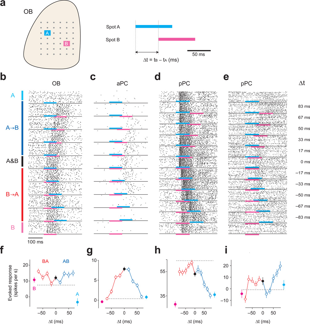
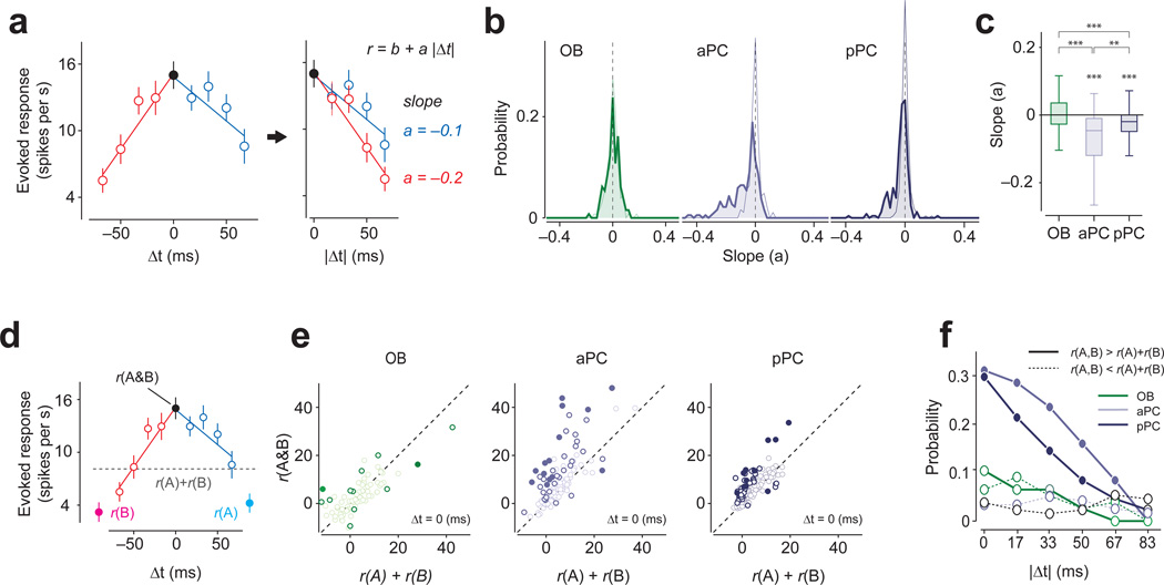
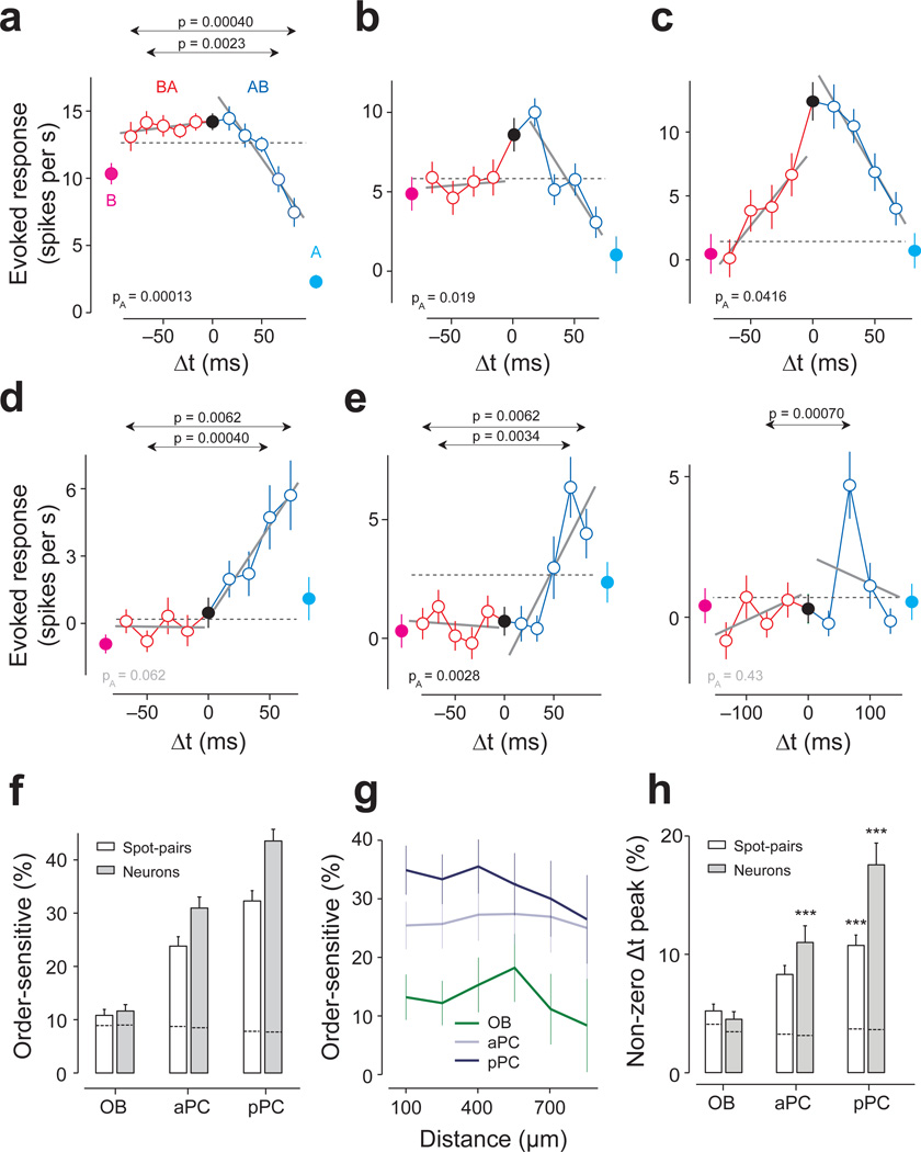
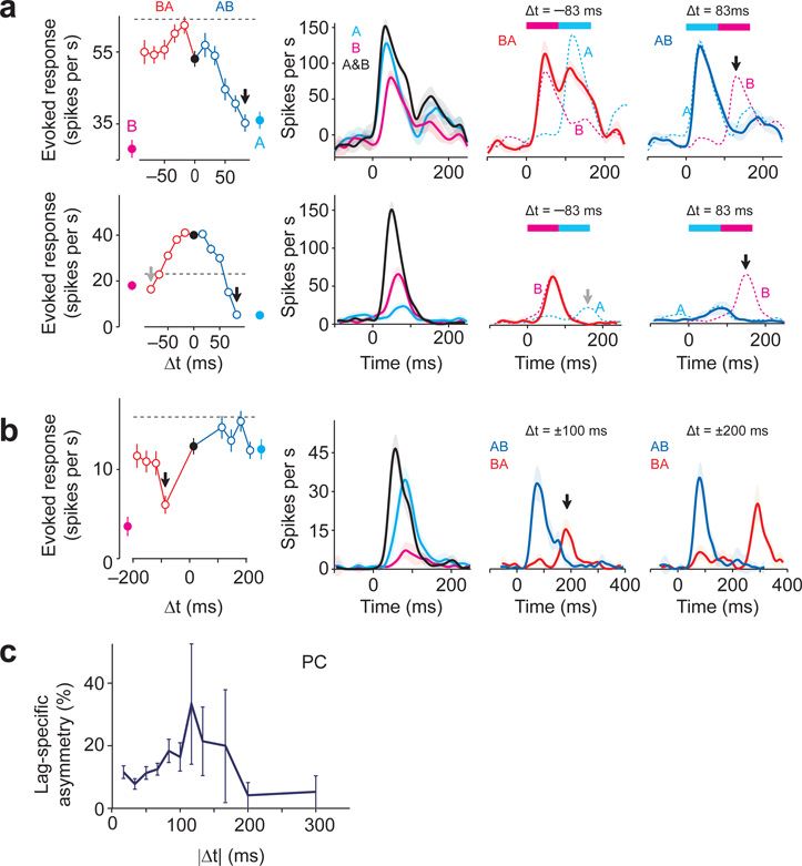
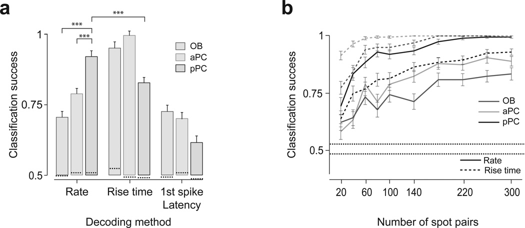
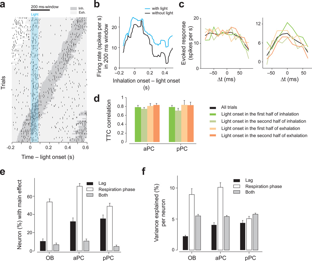
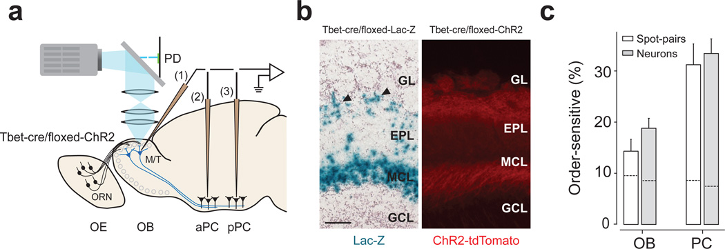
Odor stimulation evokes complex spatiotemporal activity in the olfactory bulb, suggesting that both the identity of activated neurons and the timing of their activity convey information about odors. However, whether and how downstream neurons decipher these temporal patterns remains unknown. We addressed this question by measuring the spiking activity of downstream neurons while optogenetically stimulating two foci in the olfactory bulb with varying relative timing in mice. We found that the overall spike rates of piriform cortex neurons (PCNs) were sensitive to the relative timing of activation. Posterior PCNs showed higher sensitivity to relative input times than neurons in the anterior piriform cortex. In contrast, olfactory bulb neurons rarely showed such sensitivity. Thus, the brain can transform a relative time code in the periphery into a firing rate-based representation in central brain areas, providing evidence for the relevance of a relative time-based code in the olfactory bulb.

Figure 1. Characterization of responses to single-spot, optogenetic activation of olfactory nerve input

(a) Experimental setup. Light (cyan) was focused on the surface of the olfactory bulb. Mice expressing ChR2 in ORNs were used. Spiking activity was recorded extracellularly from M/T cells in the olfactory bulb (1) and neurons in the aPC (2) and pPC (3). PD, photodiode; OE, olfactory epithelium; OB, olfactory bulb. (b) Fluorescence image of the olfactory bulb in an OMP-ChR2 mouse. Yellow indicates the location of ChR2 tagged with a yellow fluorescent protein (ChR2-YFP). ChR2 is located exclusively in the glomerular layer (GL). EPL, external plexiform layer; MCL, mitral cell layer; GRL, granule cell layer. Scale bar: 100 µm. Sections from n > 20 mice were examined. (c) Left, Two-dimensional light activation map for an example neuron in olfactory bulb. Each pixel represents the average firing rate change relative to baseline caused by activation of each olfactory bulb spot. The values are obtained using a window of 100 ms from light onset, averaged over 20-randomly interleaved repetitions. The yellow and cyan represent an increase and decrease from the baseline, respectively. The range of the scale bar corresponds to ±5 s.d. of the baseline activity. Scale bar, 150 µm. The total area scanned for an experiment was determined by the size of craniotomy. Middle and right, Peri-event time histograms (PETHs, mean ± s.e.m) and raster plots of excitatory and inhibitory spots. Each tick mark represents one spike. The timing of light stimulation is indicated by the cyan bar. The locations of the spots are indicated on the light activation map on the left. This neuron was excited by 2 spots and inhibited by 1 spot (*, t₁₉ > 2.1, P < 0.05, t-test, corrected for multiple comparisons using Bonferroni correction, n = 20 repetitions). (d) Results from an example piriform cortex neuron. An olfactory bulb was optically stimulated while a piriform cortex neuron activity was recorded. This neuron was excited by 6 spots (*, t₁₄ > 2.3, P < 0.05, t-test, Bonferroni correction, n = 15 repetitions). None of the spots caused a significant inhibitory response in this neuron. (e) Percent of excitatory spots in single-spot scanning experiments (*, P < 0.05, t-test, n = 15 – 20 repetitions, n = 29 OBNs, n = 25 aPC neurons, n = 22 pPC neurons,). The central mark indicates the median, and the edges of the box are 25^th and 75^th percentiles. Each experiment contained 42 – 60 total spots. Excitatory spots were more prevalent in aPC and pPC than in olfactory bulb (Z = 3.75, P = 0.00017; Z = 2.1; P = 0.031 for olfactory bulb versus aPC and olfactory bulb versus pPC, respectively, Mann-Whitney U test). Dashed lines inside the bars represent the FDRs. The vertical line indicates the maximum and minimum values of non-outliers. Points are considered as outliers if they are larger than b +1.5(b−a) or smaller than a −1.5(b−a), where a and b are the 25th and 75th percentiles, respectively. (f) Percent of inhibitory spots in single-spot scanning experiments as in e. Inhibitory spots were more prevalent in olfactory bulb than piriform cortex (Z = −4.6, P =3.6×10⁻⁶ and Z = −4.2, P = 1.8×10⁻⁵ for olfactory bulb versus aPC and pPC respectively, Mann-Whitney U test). Dashed lines inside the bars represent the FDRs.

Figure 2. Acquisition of temporal tuning curves (TTCs) for olfactory bulb and piriform cortex neurons

(a) Experimental design for testing temporal sensitivity. Each spot was illuminated for 83.3 ms (5 projector frames at 60Hz). Two spots in the olfactory bulb were illuminated with varying orders and lags. Lags used for the main experiment were 16, 33, 50 and 67 ms. In some experiments, larger lags were also included. For each lag, we tested the response to activation of spot A followed by B (A→B, positive Δt) and the reversed order (B→A, negative Δt). We also tested the response to each spot alone (A or B) and to simultaneous activation of the two spots (A & B, Δt = 0). (b–e) Example raster plots of one olfactory bulb (OB, b), one aPC (c) and two pPC neurons (d, e). Cyan and magenta bars indicate the timing of light stimulation of spots A and B, respectively. Each dot represents a spike, and each row represents one trial. Black lines separate between the different lags. The Δts are indicated on the right. The experiments in b and c did not include Δt = ±83 ms. (f–i) TTCs of the neurons in b-e. The total spike counts in the 200 ms analysis window were used to calculate the firing rate. The baseline firing rates in the 200 ms time window before optical stimulation were subtracted. Magenta, spot A alone; cyan, spot B alone; blue, positive Δt (A→B); red, negative Δt (B→A). Black, simultaneous stimulation of A and B (Δt = 0). Mean ± s.e.m. (n = 40 repetitions). The dashed vertical lines represent the sum of the responses to spot A alone and B alone (i.e. r(A) + r(B)).

Figure 3. Olfactory bulb and piriform cortex TTC shapes are different

(a) Analysis of TTCs. For each spot pair, two slopes were obtained by regressing the TTCs at the negative (red) and positive (blue) Δt separately with straight lines (r = b + a|Δt|). The unit of slopes is spikes/s·ms. (b) Distributions of slopes of TTCs for olfactory bulb, aPC and pPC neurons. Thin lines indicate the distribution of the slopes with the data shuffled with respect to Δts. The distribution of the slopes of the fitted lines was mostly near zero for OBNs (−0.0005 ± 0.5, t-test against zero, t₁₅₁ = 0.14, P = 0.89, n = 152 fitted lines) whereas aPC and pPC neurons’ slopes were significantly shifted below zero (aPC: −0.069 ± 0.09, t-test against zero, t₂₂₇ = 11.07, P = 4.6 × 10⁻²³n = 228 fitted lines; pPC: −0.042 ± 0.06, t₂₅₇ = 9.8, P = 1.0 × 10⁻¹⁹n = 258 fitted lines). The distribution of the slopes for OBNs was similar to those obtained in the surrogate data, suggesting that the variability in slopes originates mostly from the finite number of trials in the data. In contrast, the distribution of the slopes for PCNs was shifted compared to trial-shuffled surrogate data, and the mean slopes were significantly smaller than those of the surrogate data (P < 0.001, Kolmogorov-Smirnov test for both aPC and pPC, n = 228 and 258 fitted lines for pPC and pPC, respectively) whereas that of olfactory bulb (OB) was not (P = 0.63, Kolmogorov-Smirnov test, n = 152 fitted lines). (c) Box plots of the slopes of TTCs in the three brain regions. The mean slope of aPC and pPC neurons are significantly negative (P < 0.001 for both aPC and pPC t-test against zero). The average slope of OBNs were significantly different from those of aPC and pPC neurons (Z > 6.2, P < 3.5×10⁻¹⁰, for both olfactory bulb versus aPC and olfactory bulb versus pPC, Mann-Whitney U test,) whereas aPC slopes were also significantly different from pPC slopes (Z = −2.82, P = 0.0047, aPC versus pPC, Mann-Whitney U test,). Dashed lines represent the average slope values obtained from trial-shuffled controls in all three brain areas. The vertical line indicates the maximum and minimum values of non-outliers. Points are considered as outliers if they are larger than b +1.5(b−a) or smaller than a −1.5(b−a), where a and b are the 25th and 75th percentiles, respectively. ***, P < 0.001. (d) An example TTC to illustrate the analysis. r(A), response to A; r(B), response to B; r(A & B), response to simultaneous activation of A and B (Δt = 0). The gray dashed line indicates the arithmetic sum of the response to spot A and B (r(A) + r(B)). (e) Comparison between the sum of the responses to spots A and B (e.g. r(A) + r(B)) and the actual response for simultaneous presentation of spots A and B (r(A & B), Δt =0). Each circle represents a spot pair. Open and filled dark circles: supralinear facilitation or suppression (P < 0.05, t-test, not corrected (open) or corrected (filled) for multiple comparisons, n = 40 repetitions). In aPC and pPC neurons, the response to r(A & B) tended to be larger than r(A) + r(B). (f) Percent of spot pairs in which the responses to two-spot stimulations (r(A, B)) were greater than r(A) + r(B) (i.e. supralinear, t-test, P < 0.05, n = 40 repetitions, solid lines) or smaller (sublinear, t-test, P < 0.05, n = 40 repetitions, dashed lines) for a given lag (Δt). The average trial-shuffled control values in all three brain areas resulted in ~3% (range: 1%-8%).

Figure 4. Order-specific responses of PCNs

(a) TTC of an aPC neuron. Conventions are as in Fig. 2. The responses to B→A stimulation (red) remained flat for all lags, while the response to A→B (blue) decreased as the lag increased. This asymmetry was captured by both the global and lag-specific tests (P_A = 0.00013, F_1,446 = 14.8, ANCOVA; P = 0.0023, t₈₈ = 3.1, and P = 0.00040, t₈₈ = 3.7, t-test for Δt = ±67 and ±83 ms, respectively, n = 45 repetitions for both). Throughout the figures, P_A indicates the p-value in ANCOVA. The p-values for lag-specific comparisons are shown only when they are smaller than the criterion (t-test, corrected for the number of |Δt|’s, Bonferroni correction). Mean ± s.e.m. (b) TTC of a pPC neuron. The responses to B→A were similar to r(A) + r(B) (the gray dashed line) whereas the response for the opposite order (A→B) decreased as the lag increased. F_1,316 = 5.4, P_A = 0.019 (ANCOVA, n = 40 repetitions). (c) TTC of a pPC neuron. The responses to B→A were generally weaker than those to A→B. This asymmetry was captured by the global tests (P_A = 0.041, F_1,316 = 4.2, ANCOVA). The lag-specific differences at Δt = ±67 and ±50 ms (P = 0.023, t₇₈ = 2.3 and P = 0.025, t₇₈ = 2.3, respectively, t-test, n = 40 repetitions) did not cross the criterion (P < 0.0125; Bonferroni corrected, Supplementary Fig. 5). (d) TTC of a pPC neuron. This neuron responded maximally when spot B was stimulated 67 ms after spot A (P = 0.0055, t₇₈ = 2.8, t-test between Δt = 67 ms and Δt = 0 ms, n = 40 repetitions) and did not respond to activation of either of the spots nor to simultaneous stimulation of both spots. This asymmetry was captured by the lag-specific test (P = 0.00042, t₇₈ = 3.6 and P = 0.0062, t₇₈ = 2.8 for Δt = ±50 and ±67 ms, respectively, t-test, n = 40 repetitions for both). The global test was not significant (P_A = 0.062, F_1,316 = 3.5, ANCOVA). (e) Left, TTC of a pPC neuron. This neuron responded strongly only when A started 50–83 ms after spot B (P = 0.038, 0.00034, 0.0062, t₇₈ = 2.1, t₇₈ = 3.7, t₇₈ = 2.8 for Δt = ±50, ±66 and ±83 ms, respectively, t-test, n = 40 repetitions for all). The responses peaked at 67 ms (P = 0.00099, t₇₈ = 3.4, t-test between Δt = 67 ms and Δt = 0 ms, n = 40 repetitions).Right, TTC of the same neuron as in G₁ but tested with a different set of lags in an independent experiment. The peak at Δt = 67 ms was reproduced (P = 0.0027, t₇₈ = 3.1, t-test between Δt = −67 ms and Δt = 0 ms, n = 40 repetitions) but this experiment revealed a decrease of response with longer Δt. (f) Percentage of order-sensitive cases calculated in terms of spot pairs (white bars) and neurons (gray bars) in each brain area (Bonferonni corrected t-test for all ±Δt and P_A < 0.05, ANCOVA, n = 76, 114, 129 spot pairs and n = 45, 46, 63 neurons for olfactory bulb (OB), aPC, and pPC, respectively). Error bars, s.e.m. based on the binomial model. Dashed lines inside the bars represent the FDRs resulting in only ~8% of order-sensitive cases in all three brain areas. (g) Percentage of order-sensitive responses as a function of the distance between the spots. Error bars, s.e.m. based on the binomial model. The fraction of asymmetric TTCs in piriform cortex did not depend on the distance between the two spots as far as 1 mm on the olfactory bulb surface indicating that order-sensitive temporal interactions occur between glomeruli that are widely distributed in the olfactory bulb. This also indicates that order sensitivity is not due to an artifact caused by activation of adjacent spots through scattered light. (h) Percentage of cases in which the response to lagged stimulation (either A→B or B→A) was significantly higher than the response to A & B. The results were obtained in terms of the number of spot pairs (white bars) and neurons (gray bars). Error bars, s.e.m. based on the binomial model. Dashed lines inside the bars represent the FDRs. ***, P < 0.001 (binomial test against trial-shuffled controls, n = 76, 114, 129 spot pairs).

Figure 5. Delayed inhibition shapes the responsivity of PCNs

(a) Upper panel, TTC of an example pPC neuron. The same neurons as in Fig. 2d, h. Second panel, PETHs of the responses. The response decreased steeply with increasing Δt for A→B but not for B→A. Middle panel, Δt = −83 ms; right panel, Δt = 83 ms. Dashed lines in the right two panels represent expected firing rate changes in response to the corresponding spot (A or B). The second stimulation was effective in evoking responses with Δt = 83 ms (third panel), but not with Δt = −83 ms (fourth panel, black arrow). Lower panel, TTC of a pPC neuron. With Δt = ±83 ms, the response to A→B differed significantly from that of B→A (left panel, black and gray arrows). Note that second spot stimulation did not elicit the expected responses in both orders (third and fourth panels, black and gray arrows). (b) TTC of a pPC neuron which was tested with longer lags (Δt = 100, 133, 167 and 200 ms). The TTC is asymmetric at Δt = ±100 ms (black arrow, P = 0.000023, t₇₈ = 4.5, t-test, n = 40 repetitions) but similar for Δt = 200 ms (P = 0.72, t-test, t₇₈ = 0.36). With Δt = −100 ms, stimulation of the second spot A does not elicit a strong response (third panel, B→A, red line and black arrow). However, with a larger lag (Δt = ±200 ms), the response to spot A resumed (red line in the fourth panel). (c) Percentages of lag-specific asymmetry in TTCs for each lag for all PCNs. Mean ± s.e.m. based on the binomial model.

Figure 6. Rate code conveys relative timing information progressively more at the central areas

(a) Classification success rates based on three different decoding methods. A linear classifier was trained to classify the neuronal responses of a population of neurons as belonging to either positive or negative Δt. A classifier was first trained using all but 10% of the trials including all Δt, and the remaining 10% of the trials were used to test the performance of the classifier (a leave-10%-out procedure). The result was obtained using neural activity representing 100 spot pairs randomly sampled from the data obtained from 45, 47 and 63 neurons in olfactory bulb (OB), aPC and pPC, respectively (see Methods). The mean classification success rate was obtained from 500 repetitions using different random sets of test trials. Rate code is based on the number of spikes evoked in the analysis window of 200 ms. Rise time code is based on the time at which the number of spikes in a window of 20 ms became ±2 s.d. higher (or lower) than the baseline. Latency to first spike time is defined as the time of the first spike from stimulation onset. ***, P < 0.001 (binomial test). Mean ± s.e.m. Dashed lines inside the bars represent the FDRs. (b) Classification success rates as a function of the number of spot pairs. Mean ± s.e.m. (n = 500 repeats). The lower and upper dashed lines represent the minimum and maximum FDRs.

Figure 7. Order-selectivity is largely preserved across different respiration phases

(a) Raster plot of an M/T cell in response to single spot optical stimulation. Each tick mark represents one spike. The dark gray area indicates inhalation periods and the light gray areas exhalation periods. Trials are sorted by the timing of inhalation onset. The timing of light stimulation (duration: 83 ms) is indicated by the cyan area. This neuron fired preferentially during inhalation periods. (b) Firing rates in a 200 ms window (indicated at the top of A) as a function of inhalation onset timing relative to light onset (cyan). The data with no light stimulation (black) was obtained by randomly assigning light onset relative to the respiration cycle. (c) Two examples comparing TTCs at specific respiration phases. The data were parceled into four groups depending on the onset of light stimulation (as indicated in d). Green: trials in which the light started in the first half of the inhalation. Light green: trials in which the light started in the second half of the inhalation. Light orange: trials in which the light started in the first half of the exhalation. Orange: trials in which the light started in the second half of the exhalation. Black: all trials. The shapes of TTCs were similar across the four groups. (d) Correlation of TTCs. A TTC was obtained for each of the four groups as in c. The correlation between this TTC and the TTC computed with all other trial groups was obtained. The bar graphs show the median correlation across all spot pairs in each brain area. TTCs were obtained only if at least 10 trials were available for all of the four groups. n = 112 and 95 TTCs for aPC and pPC, respectively Mean ± s.d.. (e) Percent of neuron-spot pairs that were modulated by the lag and/or the respiration phase (two-way ANOVA, F_3,199 > 2.6 or/and F_4,199 > 2.4, P < 0.05, for 4 and 5 Δt, respectively, uncorrected for multiple comparisons. Many neurons were modulated by the respiration phase (white bars). Many neurons in aPC and pPC were modulated by the lag between two spot activations but neurons in olfactory bulb were not (black bars; binomial test, P < 0.001 for both aPC and pPC compared to olfactory bulb [OB]). Error bars: s.e.m. based on the binomial model. The number of TTCs used in the analysis was 134, 224, 190 in the olfactory bulb, aPC and pPC respectively. (f) The variance of neural responses explained by different factors per neuron (two-way ANOVAs, the average variance explained by the lag, respiration phase or both). Respiration phase explains on average ~10% of the variance in olfactory bulb and aPC. The lag between spot activations explain more of the variance in PCNs than in OBNs (Z = −3.2, P = 0.0011 and Z = −4.3, P = 0.000016 for aPC and pPC compared to olfactory bulb respectively, Mann-Whitney U test). Mean ± s.e.m.. n = 134, 224 and 190 TTCs in the olfactory bulb, aPC and pPC, respectively.

Figure 8. Direct activation of M/T cells produced consistent results

(a) Experimental design. Conventions are as in Fig. 1a. (b) Characterization of Tbet-cre/floxed-ChR2 mouse. Left, a section from a Tbet-cre/floxed-Lac-Z mouse. Blue signals (lacZ staining) depict the location of cell bodies. Mitral and tufted cells (arrowheads) are stained. Right, fluorescent image of an olfactory bulb section. Red indicates the location of ChR2 tagged with a red fluorescent protein (tdTomato). Sections from n = 2 and n > 20 mice were examined for lacZ staining and tdTomato fluorescence, respectively. GL: glomerular layer; EPL, external plexiform layer; MCL, mitral cell layer; GRL, granule cell layer. OB, olfactory bulb. Scale bar: 100 µm. (c) Percentage of order-sensitive responses in olfactory bulb (n = 17 neurons and 28 responding spot pairs) and PCNs (n = 34 neurons and 67 responding spot pairs). The results were obtained in terms of spot pairs (white bars) and neurons (gray bars). The data from aPC and pPC were pooled. Dashed lines inside the bars represent the FDRs.

References

1. Adrian ED. The impulses produced by sensory nerve endings: Part I. J Physiol. 1926;61:49–72. - PMC - PubMed
1. Wehr M, Laurent G. Odour encoding by temporal sequences of firing in oscillating neural assemblies. Nature. 1996;384:162–166. - PubMed
1. VanRullen R, Guyonneau R, Thorpe SJ. Spike times make sense. Trends Neurosci. 2005;28:1–4. - PubMed
1. Laurent G. A systems perspective on early olfactory coding. Science. 1999;286:723–728. - PubMed
1. Hopfield JJ. Pattern recognition computation using action potential timing for stimulus representation. Nature. 1995;376:33–36. - PubMed
Publication types
MeSH terms
LinkOut - more resources