Space can substitute for time in predicting climate-change effects on biodiversity

Abstract

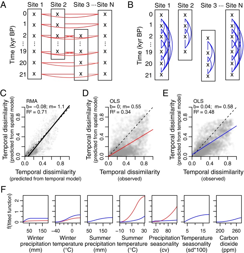
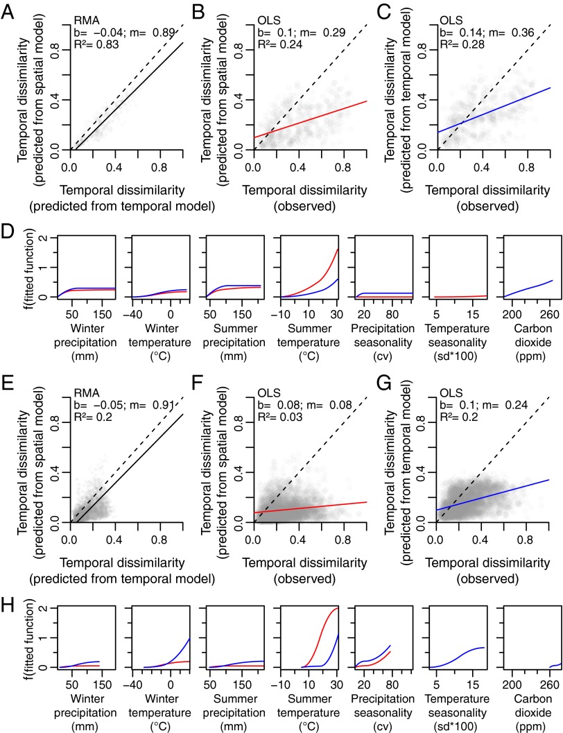
"Space-for-time" substitution is widely used in biodiversity modeling to infer past or future trajectories of ecological systems from contemporary spatial patterns. However, the foundational assumption--that drivers of spatial gradients of species composition also drive temporal changes in diversity--rarely is tested. Here, we empirically test the space-for-time assumption by constructing orthogonal datasets of compositional turnover of plant taxa and climatic dissimilarity through time and across space from Late Quaternary pollen records in eastern North America, then modeling climate-driven compositional turnover. Predictions relying on space-for-time substitution were ∼72% as accurate as "time-for-time" predictions. However, space-for-time substitution performed poorly during the Holocene when temporal variation in climate was small relative to spatial variation and required subsampling to match the extent of spatial and temporal climatic gradients. Despite this caution, our results generally support the judicious use of space-for-time substitution in modeling community responses to climate change.

Keywords: fossil pollen; generalized dissimilarity modeling; global change; paleoecology.

Fig. 1.

Spatial (A) and temporal (B) dataset construction, resulting predictions of temporal turnover (C–E), and fitted functions (F) for the Late Quaternary datasets (21–0 kyBP). In all cases, the red lines indicate spatial datasets, blue lines indicate temporal datasets, and dashed lines indicate the 1:1 line. (C) RMA regression between temporal turnover predicted by the temporal model and by the spatial model. (D) OLS regression between observed temporal turnover and temporal turnover predicted by the spatial model (space-for-time substitution). (E) OLS regression between observed temporal turnover and temporal turnover predicted by the temporal model (time-for-time substitution). (F) The fitted functions for each variable. b, Intercept of the regression line; cv, coefficient of variation; m, slope of the regression line; R², goodness of fit.

Fig. 2.

Predictions and fitted functions for the Late Pleistocene (21–11 kyBP) (A–D) and the Holocene (10–0 kyBP) (E–H). In all cases, the red lines indicate spatial datasets, blue lines indicate temporal datasets, and dashed lines indicate the 1:1 line. (A and E) Model-to-model RMA regression between temporal turnover predicted from the temporal model and from the spatial model. (B and F) Space-for-time OLS regression between observed temporal turnover and temporal turnover predicted from the spatial model. (C and G) Time-for-time OLS regression between observed temporal turnover and temporal turnover predicted from the temporal model. (D and H) Fitted functions for the spatial and temporal models. Abbreviations are as in Fig. 1.

Fig. 3.

Range of climate dissimilarity and model predictions for the Late Pleistocene (21–11 kyBP) (A–E) and Holocene (10–0 kyBP) (F–J). Light gray indicates the unsampled datasets, red indicates the climate-subsampled spatial datasets, and blue indicates the climate-subsampled temporal datasets. (A and F) Euclidean climate dissimilarity for the spatial datasets. (D and I) Euclidean climate dissimilarity for the temporal datasets. (B and G) Space-for-time OLS regression between observed temporal turnover and temporal turnover predicted by the spatial model. (E and J) Time-for-time OLS regression between observed temporal turnover and temporal turnover predicted by the temporal model. (C and H) Model-to-model RMA regression between temporal turnover predicted by the temporal model and by the spatial model for the climate-subsampled dataset (dark gray) and the unsampled dataset. Regression statistics for analyses based on the climate-subsampled datasets are indicated for each scatter plot. Abbreviations are as in Fig. 1.

References

1. Fastie CL. Causes and ecosystem consequences of multiple pathways of primary succession at Glacier Bay, Alaska. Ecology. 1995;76(6):1899–1916.
1. Johnson EA, Miyanishi K. Testing the assumptions of chronosequences in succession. Ecol Lett. 2008;11(5):419–431. - PubMed
1. Pickett S. Space-for-time substitution as an alternative to long-term studies. In: Likens GE, editor. Long-Term Studies in Ecology: Approaches and Alternatives. New York: Springer; 1989. pp. 110–135.
1. Imbrie J, Kipp NG. A new micropaleontological method for quantitative paleoclimatology: Application to a late Pleistocene Caribbean core. In: Turekian K, editor. The Late Cenozoic Glacial Ages. New Haven, CT: Yale Univ Press; 1971. pp. 77–181.
1. Tierney JE, et al. Environmental controls on branched tetraether lipid distributions in tropical East African lake sediments. Geochim Cosmochim Acta. 2010;74(17):4902–4918.
Publication types