

doi: 10.1080/09291010600903692.
Procedures for numerical analysis of circadian rhythms
Affiliations
- PMID: 23710111
- PMCID: PMC3663600
- DOI: 10.1080/09291010600903692
Item in Clipboard
Procedures for numerical analysis of circadian rhythms
Biol Rhythm Res.
2007.
Abstract
This article reviews various procedures used in the analysis of circadian rhythms at the populational, organismal, cellular and molecular levels. The procedures range from visual inspection of time plots and actograms to several mathematical methods of time series analysis. Computational steps are described in some detail, and additional bibliographic resources and computer programs are listed.
Keywords: Biostatistics; chronobiology; chronomics; circadian rhythm; time series analysis.
Figures

Treatment of perioral cancer timed at peak tumor temperature leads to more than doubling of the 24-month survival rate, as compared to reference groups treated 4 or 8 hours before or after the tumor temperature peak. The dashed line indicates the outcome for treatment conducted without regard for circadian time. Data from Halberg et al. (2003a), as documented by a peak test (Savage et al. 1962).

Flowchart of some of the methods available for analysis in chronobiology and for chronomics, with emphasis on extended cosinor rhythmometry. Note on the top of the chart that one can start with a time-specified datum as well as with a time series. This is because the methods of rhythmometry also serve for the preparation of reference intervals. Such time-specified reference intervals, or chronodesms, and their variants are currently a raison d’être of clinical chronobiology, as this discipline resolves the normal range of variation. Use of the procedures outlined in this flowchart has to be based on cost-effectiveness that determines the sampling requirements which in research will be much more demanding for exploring new periodicities even in the circadian spectral region than for dealing with already-mapped rhythms. As biology and medicine involve longer and longer series, it will become essential to resolve more than single components in a given spectral region, including the circadian one. As more and more variables can be studied concomitantly for long spans, procedures that analyze relations among time series will become indispensable. Adapted from Halberg et al. (1987).

Diagram illustrating aliasing (that is, identification of a spurious “rhythm” [alias] because of poor [insufficiently dense] sampling of an actual rhythmic process). The actual rhythmic component in this graph is sinusoidal with a period of 27.43 h. Sampling once a day at a fixed clock hour is shown by the dots. Analysis of the sampled data detects a component with a period of 8 days instead of 27.43 h. More generally, aliasing refers to all artifacts resulting from insufficiently dense sampling that fails to detect rhythm characteristics, such as the amplitude, acrophase or waveform (as well as the period illustrated on this graph). Adapted from Halberg et al. (1977).

Time plots of the records of body temperature of a gerbil collected by radio-telemetry every 6 minutes for 8 consecutive days (A) and of a simulated data set containing temperature values sampled in the same temperature range but temporally randomized (B). An approximately 24-h pattern of oscillation is evident in A but not in B. Data from Refinetti (1998).

Actogram of the running-wheel activity rhythm of a Nile grass rat recorded with 6-min resolution for 35 consecutive days. As indicated by the horizontal bars at the top, a light – dark cycle was in effect for the first 22 days (LD), whereas darkness prevailed for the following 13 days (DD). The rhythm free-ran in constant darkness with a period shorter than 24.0 h. Data from Refinetti (2004a).

Temporal distributions of suicides. (A) Accumulated temporal distribution of train suicides in the Netherlands from 1980 to 1994 (data from Houwelingen & Beersma 2001). (B) Distribution of values sampled in the same range as in A but temporally randomized. (C) Longitudinal data on suicides in Minnesota from 1968 to 2002 shown as monthly means (data from Halberg et al. 2005). (D) Subset of the Minnesota data set showing the number of daily suicides during the first two months of 2001. (E) Spectrum of cosinor amplitudes for the full time series (1968 – 2002).

Mean concentration of cholesterol in the serum of a goat sampled every 3 h for 10 consecutive days (A) and simulated data set with randomized time bins (B). Each vertical bar indicates the mean (+SE) of the 10 measurements conducted at each of the eight daily collection times. The horizontal bar at the top indicates the duration of the light and dark phases of the prevailing light-dark cycle. Analysis by ANOVA rejects the hypothesis of uniformity in both cases, but only A exhibits 24-h rhythmicity. Data from Piccione et al. (2003).

Records of locomotor activity of a horse monitored by actigraphy at 1-min intervals for 10 consecutive days (top) and the periodogram generated by Fourier analysis of the time series (bottom). The dashed line in the periodogram indicates the 0.05 level of significance. Visual inspection of the raw data suggests the existence of 24-h rhythmicity, and the Fourier periodogram confirms it by showing a large peak at 24.0 h. Other, smaller peaks can also be seen (arrows). Data from Piccione et al. (2005).

Educed rhythm of systolic blood pressure of a healthy woman collected at irregular intervals over nine days (points) and cosine wave fitted by the method of the least squares (curve). The small rectangle denotes the width of the 95% confidence interval of curve fitting. Data from Cornélissen and Halberg (2005).

Expression of the per1 gene in liver and testis of mice. Each data point corresponds to the mean (+SE) of three mice. The dashed lines indicate the overall means for the whole data sets. The rectangles denote the width of the 95% confidence intervals of curve fitting. The confidence interval overlaps the mean in the testis but not in the liver. Data from Yamamoto et al. (2004).

Temporal distribution of activity onsets of Siberian hamster pups a few days after weaning. Each dot denotes one pup. (A) uniform distribution; (B) actual distribution. The estimated time of the activity onset of the dams (time 12 of the LD cycle preceding constant darkness) is indicated by the arrowhead. Data from Duffield and Ebling (1998).

Ten-day segment of the records of running-wheel activity of a mouse maintained under a 24-h light-dark cycle and three periodograms generated by analysis of these data. The dashed lines in the periodograms indicate the 0.01 level of significance. Visual inspection of the time plot suggests the presence of strong rhythmicity with a period of 24.0 h. The three periodograms support this interpretation. Data from Refinetti (2004a).

Probability under the null hypothesis (Ho) as a function of the signal-to-noise ratio of the data sets for tests of 24.0-h rhythmicity conducted by Fourier analysis, by the cosinor procedure, by the Enright periodogram, and by the Lomb – Scargle periodogram. The horizontal line indicates p =0.05. The cosinor procedure detected significant rhythmicity in data sets with signal-to-noise ratios as low as 0.01 (1% signal and 99% noise).

Diagram of an oscillatory process identifying four parameters of the oscillation: mesor, period, amplitude, and phase.

Diagram depicting oscillations with different waveforms (A-C), unstable period (D), unstable waveform (E), and linear trend (F).

Artificial data sets of square waves with periods of 12, 24, and 48 h (left column) and their analyses by the chi square periodogram (QP) and the Lomb – Scargle periodogram (PN). The dashed lines in the periodograms indicate the 0.001 level of significance. The chi square periodogram identified a large 24 h component in the data set that contained only a 12-h square wave. Both methods correctly identified the 24-h component of the 24-h wave, although the Lomb – Scargle periodogram erroneously identified other smaller components (arrows). The chi square periodogram correctly failed to identify circadian rhythmicity in the 48-h wave, whereas the Lomb – Scargle periodogram identified a small 16-h component (arrow), which corresponds to the third harmonic of the 48-h component.

Periodograms describing sinusoidal time series with periods of 24 h. Fourier analysis (A) and chi square periodogram (B) were used to analyze segments of a time series generated with temporal resolution of 6 minutes. Notice that greater resolution of analysis is attained for longer segments of the time series. Lomb – Scargle periodogram (C) was used to analyze 10-day segments of times series generated with different temporal resolutions. Notice that statistical power (as indicated by the fraction of the curve above the significance line), but not resolution of analysis, is greater when the resolution of the data is greater. Notice also that the level of the line indicating statistical significance changes as a function of the number of degrees of freedom, which increases with the number of data available as the sampling interval gets shorter.

Periodograms describing time series containing two sinusoidal components: 21.0 and 25.0 h (A) or 23.5 and 24.5 h (B). In A, but not in B, the Enright (chi square) and Lomb – Scargle periodograms provide better visualization of the two components than does the Fourier periodogram.
An artificial data set lasting 14 days with hourly observations. The data set, which contains a large 24.0-h component and a smaller 24.8-h component, was constructed according to Yi =100 + 10 cos (2πti/24−π) + 2 cos (2πti/ 24.8−π) + 5 R, where i =1, . . . , 336 (Δt =1 h) and R is uniformly distributed with zero mean and range =1 (±0.5).

Advantages of the MESOR over the arithmetic mean in the estimation of central tendency of a time series. (A) the MESOR has smaller bias in the presence of unequidistant data. (B) the standard error (SE) of the MESOR reflects the variability of the data after the variability accounted for by the rhythmic pattern has been removed. It differs from the global SE reflecting the total variability of the data (most of which can be ascribed to the rhythmic time structure). From Cornélissen et al. (1999). © Halberg. Reproduced with permission.

Analysis by a moving cosinor of phase-shifting of circadian rhythms in oral temperature of five healthy adult white males following transmeridian flights in two directions. Adapted from Halberg (1969).

Polar representation of the amplitude and acrophase of a rhythm, as computed by the cosinor method. The acrophase (φ) is indicated by the angle of a vector whose length corresponds to the amplitude (A). The ellipse denotes the 95% confidence region for the joint estimation of A and φ. Conservative estimates of 95% confidence intervals for A and φ alone can be obtained by drawing concentric circles tangent to the error ellipse for A, determining their intersection with the vector’s length (A), or by drawing tangents to the ellipse for φ.
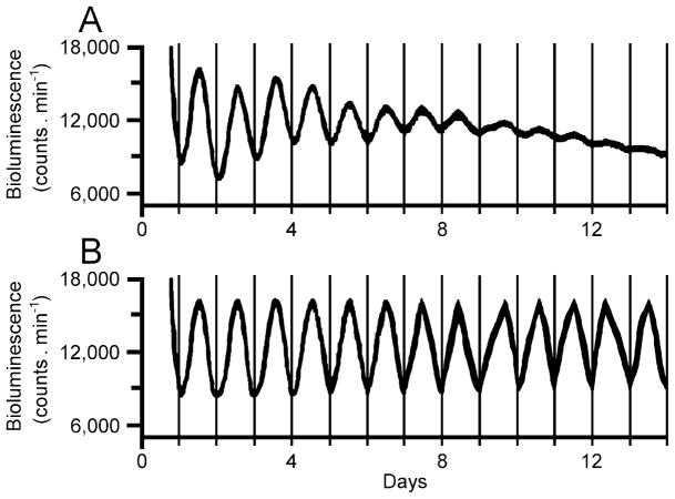
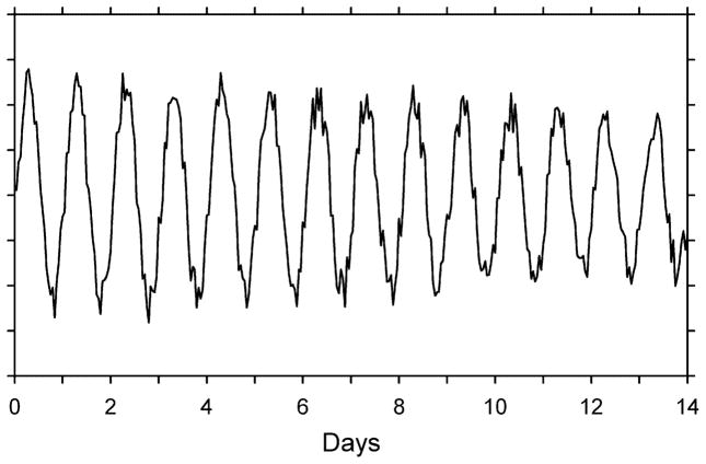
Two-week segments of the records of bioluminescence of cells in the suprachiasmatic nucleus of a mouse culture in vitro. Because of suboptimal culturing conditions, the rhythm of bioluminescence showed a reduction in amplitude and mesor during the recording interval. (A) original data; (B) filtered data. Data from Yoo et al. (2004).

Graphic display of temporal pattern of gene expression of a sub-sample of 1,104 genes (out of a total of 14,010 genes) from a DNA microarray study conducted on fruit flies. Samples of RNA were collected at 4 h intervals from flies maintained under a light – dark cycle. Different levels of gene expression (normalized for each gene) are denoted by different shades of grey. Many genes exhibit variation in expression along the day. Data from Lin et al. (2002).

Diagram to guide the selection of procedures for the detection of circadian rhythmicity.

Blunders from time-unspecified comparisons of groups characterized by a difference in amplitude, acrophase or period but not in MESOR are best avoided by including the assessment of rhythms in the design of studies and by assessing all rhythm characteristics. Measurements conducted at arbitrary time points in ignorance of rhythmicity can lead to opposite conclusions about the characteristics of processes A and B.

Confusing results, that could wrongly be interpreted as “stress” or “allergy”, are accounted for by the action of food (offered mornings) and light as competing synchronizers of circadian rhythms in counts of circulating eosinophils in C3H mice with high breast cancer incidence that can be drastically reduced by calorie restriction. Apart from constituting the beginning of Minnesotan chronobiology, and beyond the demonstration that time-unspecified spotchecks must not underlie frequently made inferences of “up-” and “down-regulation”, these studies convey the need to rely on circadian rhythms (and even broader time structures, chronomes) as the indispensable control information for any rhythmic variable, and hence the need to complement the mapping of genomes with the mapping of chronomes. From Halberg et al. (2003b). © Halberg. Reproduced with permission.
Similar articles
-
'Chronomics' in ICU: circadian aspects of immune response and therapeutic perspectives in the critically ill.Intensive Care Med Exp. 2014 Dec;2(1):18. doi: 10.1186/2197-425X-2-18. Epub 2014 May 14. Intensive Care Med Exp. 2014. PMID: 26266918 Free PMC article.
-
Bibliometric and visual analysis of circadian rhythms in depression from 2004 to 2024.Ann Gen Psychiatry. 2025 May 14;24(1):27. doi: 10.1186/s12991-025-00565-x. Ann Gen Psychiatry. 2025. PMID: 40369622 Free PMC article.
-
Circadian rhythmicity of body temperature and metabolism.Temperature (Austin). 2020 Apr 17;7(4):321-362. doi: 10.1080/23328940.2020.1743605. eCollection 2020. Temperature (Austin). 2020. PMID: 33251281 Free PMC article. Review.
-
Ethical and methodological standards for laboratory and medical biological rhythm research.Chronobiol Int. 2008 Nov;25(6):999-1016. doi: 10.1080/07420520802544530. Chronobiol Int. 2008. PMID: 19005901
-
Postoperative circadian disturbances.Dan Med Bull. 2010 Dec;57(12):B4205. Dan Med Bull. 2010. PMID: 21122464 Review.
Cited by
-
Photoperiodic influences on ultradian rhythms of male Siberian hamsters.PLoS One. 2012;7(7):e41723. doi: 10.1371/journal.pone.0041723. Epub 2012 Jul 27. PLoS One. 2012. PMID: 22848579 Free PMC article.
-
Desoxycorticosterone pivalate-salt treatment leads to non-dipping hypertension in Per1 knockout mice.Acta Physiol (Oxf). 2017 May;220(1):72-82. doi: 10.1111/apha.12804. Epub 2016 Oct 3. Acta Physiol (Oxf). 2017. PMID: 27636900 Free PMC article.
-
Seizure-related differences in biosignal 24-h modulation patterns.Sci Rep. 2022 Sep 5;12(1):15070. doi: 10.1038/s41598-022-18271-z. Sci Rep. 2022. PMID: 36064877 Free PMC article.
-
Seasonal patterns of body temperature in response to experimental photoperiod variation in a non-hibernating ground squirrel.J Comp Physiol B. 2023 Mar;193(2):219-226. doi: 10.1007/s00360-023-01477-6. Epub 2023 Feb 25. J Comp Physiol B. 2023. PMID: 36840751
-
Daily rhythms of rectal and body surface temperatures in donkeys during the cold-dry (harmattan) and hot-dry seasons in a tropical savannah.Int J Biometeorol. 2018 Dec;62(12):2231-2243. doi: 10.1007/s00484-018-1626-z. Epub 2018 Oct 29. Int J Biometeorol. 2018. PMID: 30374600
References
-
- Akiyama T. Entrainment of the circatidal swimming activity rhythm in the cumacean Dimorphostylis asiatica (Crustacea) to 12.5-hour hydrostatic pressure cycles. Zool Sci. 2004;21:29–38. - PubMed
-
- Albers HE, Gerall AA, Axelson JF. Effect of reproductive state on circadian periodicity in the rat. Physiol Behav. 1981;26:21–25. - PubMed
-
- Albert PS. On analyzing circadian rhythms data using nonlinear mixed models with harmonic terms. Biometrics. 2005;61:1115–1120. - PubMed
-
- Almirall H. Modeling the body temperature throughout the day with a two-term function. Behav Res Methods Instrum Comput. 1997;29:595–599.
-
- Alonso I, Fernández JR. Nonlinear estimation and statistical testing of periods in nonsinusoidal longitudinal time series with unequidistant observations. Chronobiol Int. 2001;18:285–308. - PubMed
Grants and funding
LinkOut - more resources
Full Text Sources
Other Literature Sources