Bayesian analysis of biogeography when the number of areas is large

Abstract

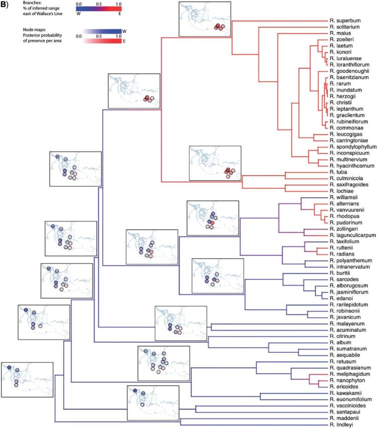
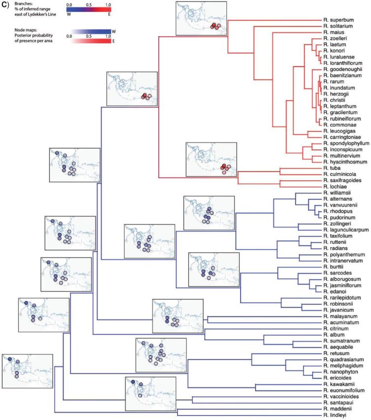
Historical biogeography is increasingly studied from an explicitly statistical perspective, using stochastic models to describe the evolution of species range as a continuous-time Markov process of dispersal between and extinction within a set of discrete geographic areas. The main constraint of these methods is the computational limit on the number of areas that can be specified. We propose a Bayesian approach for inferring biogeographic history that extends the application of biogeographic models to the analysis of more realistic problems that involve a large number of areas. Our solution is based on a "data-augmentation" approach, in which we first populate the tree with a history of biogeographic events that is consistent with the observed species ranges at the tips of the tree. We then calculate the likelihood of a given history by adopting a mechanistic interpretation of the instantaneous-rate matrix, which specifies both the exponential waiting times between biogeographic events and the relative probabilities of each biogeographic change. We develop this approach in a Bayesian framework, marginalizing over all possible biogeographic histories using Markov chain Monte Carlo (MCMC). Besides dramatically increasing the number of areas that can be accommodated in a biogeographic analysis, our method allows the parameters of a given biogeographic model to be estimated and different biogeographic models to be objectively compared. Our approach is implemented in the program, BayArea.

Figure 1

An example of a tree with M = 4 species. A) Nodes on the tree are labeled such that the tips of the tree have the labels 1,2,...,M whereas the interior nodes of the tree are labeled M +1,M +2,...,2M. Note that in this article we also consider the “stem” branch of the tree, which connects the root node (node 7) and its immediate common ancestor (node 8). B–D) Several possible biogeographic histories—comprising 6, 6, and 12 events, respectively—that can explain the observed species ranges.

Figure 2

Cartoon of the computation of the distance-dependent dispersal-rate modifier, η(·). Here, we are interested in computing the rate of y = 1100 transitioning to z = 1101. The first term computes the sum of inverse distances raised to the power β between the area of interest (i.e., 4) and all currently occupied areas (i.e., areas 1 and 2). The second term then normalizes this quantity by dividing by the sum of inverse distances raised to the power β between all occupied–unoccupied area-pairs (i.e., the denominator), then multiplying by number of currently unoccupied areas (i.e., 2, the numerator).

Figure 3

Cartoon of the likelihood terms. The biogeographic history for lineage i includes the lineage start at time τ₁⁽ⁱ⁾, an extinction event at area 2 at time τ₂⁽ⁱ⁾, a dispersal event into area 3 at time τ₃⁽ⁱ⁾, and the lineage end at time τ_F⁽ⁱ⁾, with all events laying within the time interval (3.2,9.3). The probability of a sampled geographic range at the start of the branch is conditioned on the previous (ancestral) geographic range and the time separating the geographic ranges, Δτ_k⁽ⁱ⁾ = τ_k−1⁽ⁱ⁾ − τ_k⁽ⁱ⁾. The likelihood is the product of the probabilities corresponding to each interval accounting for an area loss at time τ₂⁽ⁱ⁾, an area gain at time τ₃⁽ⁱ⁾, and no further changes occurring before the lineage terminates.

Figure 4

Distributions of means of posteriors of simulation study. Fifty data sets were simulated for each value of β ∈ {0,0.25,0.5,1,2,3,4,6} while λ₀ = 0.05 and λ₁ = 0.005 were held constant. For each set of 50 data sets, the mean of the posterior of each parameter was computed under the distance-dependent dispersal model. Distribution means are given by a bold line, while the 25th and 75th percentiles are given by the lower and upper edges of each box, called Q1 and Q3, respectively. The upper and lower whiskers indicate Q1 − IQR and Q3 + IQR, where IQR = 1.5 × (Q3 − Q1), and circles indicate outliers. The true parameter values are given by (A,B) the horizontal dashed line, and (C) the squares.

Figure 5

Distributions of Bayes factors for the simulation study. Fifty data sets were simulated for each value of β ∈ {0,0.25,0.5,1,2,3,4,6} while λ₀ = 0.05 and λ₁ = 0.005 were held constant. Columns display the frequencies of strengths of support in favor of the distance-despendent dispersal model, where strengths of support correspond to the intervals suggested by Jeffreys (1961): Favors ℳ₀ on (−∞, 1); Insubstantial on [1, 3); Substantial on [3,10); Strong on [10,30); Very strong on [30,100); Decisive on [100,8). Each column corresponds to the strengths of support per 50 β-valued simulations. Bayes factors generally select the correct underlying model except for β = 0.25.

Figure 6

Errors for inferred dispersal histories of simulation study. The sum of squared differences between the posterior probability (i.e., 0 < P < 1) and the true history (i.e., P = 0 or P = 1) for each area and each internal node were computed per simulated data set. The box plots show the distribution of these sums for each batch of 50 simulated data sets per value of β ∈ {0,0.25,0.5,1,2,3,4,6}. Distribution means are given by a bold line, while the 25th and 75th percentiles are given by the lower and upper edges of each box, called Q1 and Q3, respectively. The upper and lower whiskers indicate Q1 − IQR and Q3 + IQR, where IQR = 1.5 × (Q3 − Q1), and circles indicate outliers.

Figure 7

Marginal posterior densities for dispersal parameters from the Malesian Rhododendron data set. MAP values (dashed gray line) for the distance-dependent dispersal model parameters are A) λ₀ = 0.13, B) λ₁ = 0.013; and C) β = 2.65. The dotted black line corresponds to the prior, β ~ Cauchy(0,1). Note that the posterior probability of β = 0 is ~ 0, resulting in “Decisive” support (c.f., Jeffreys 1961) for the distance-dependent dispersal model over the mutual-independence model.

Figure 8

Biogeographic history of Malesian Rhododendron. A) The region was parsed into 20 discrete geographic areas following Brown et al. (2006), which straddle two important biotic boundaries—Wallace's and Lydekker's Lines. Each circle corresponds to a discrete area. Distances between these areas are based on a single coordinate for each area, indicated by an “x”. Posterior probability of being present in an area is proportional to the opacity of the circle. Occupied areas with posterior probabilities < 0.12 are masked to ease interpretation. Circles are shaded according to their position relative to Wallace's Line (B) or Lydekker's Line (C). Branches are shaded by a gradient representing the sum of posterior probabilities of being present per area for descendant–ancestor pairs. We infer a continental Asian origin for Malesian rhododendrons with multiple dispersal events across Wallace's Line (B) and a single dispersal event across Lydekker's Line (C).

Figure 8

Biogeographic history of Malesian Rhododendron. A) The region was parsed into 20 discrete geographic areas following Brown et al. (2006), which straddle two important biotic boundaries—Wallace's and Lydekker's Lines. Each circle corresponds to a discrete area. Distances between these areas are based on a single coordinate for each area, indicated by an “x”. Posterior probability of being present in an area is proportional to the opacity of the circle. Occupied areas with posterior probabilities < 0.12 are masked to ease interpretation. Circles are shaded according to their position relative to Wallace's Line (B) or Lydekker's Line (C). Branches are shaded by a gradient representing the sum of posterior probabilities of being present per area for descendant–ancestor pairs. We infer a continental Asian origin for Malesian rhododendrons with multiple dispersal events across Wallace's Line (B) and a single dispersal event across Lydekker's Line (C).

Figure 8

Biogeographic history of Malesian Rhododendron. A) The region was parsed into 20 discrete geographic areas following Brown et al. (2006), which straddle two important biotic boundaries—Wallace's and Lydekker's Lines. Each circle corresponds to a discrete area. Distances between these areas are based on a single coordinate for each area, indicated by an “x”. Posterior probability of being present in an area is proportional to the opacity of the circle. Occupied areas with posterior probabilities < 0.12 are masked to ease interpretation. Circles are shaded according to their position relative to Wallace's Line (B) or Lydekker's Line (C). Branches are shaded by a gradient representing the sum of posterior probabilities of being present per area for descendant–ancestor pairs. We infer a continental Asian origin for Malesian rhododendrons with multiple dispersal events across Wallace's Line (B) and a single dispersal event across Lydekker's Line (C).

References

1. Brown G., Nelson G., Ladiges P.Y. Historical biogeography of Rhododendron Section Vireya and the Malesian Archipelago. J. Biogeogr. 2006;33:1929–1944.
1. Buerki S., Forest F., Alvarez N., Nylander J.A.A., Arrigo N., Sanmartín I. An evaluation of new parsimony-based versus parametric inference methods in biogeography: a case study using the globally distributed plant family Sapindaceae. J Biogeog. 2011;38:531–550.
1. Carlquist S. The biota of long-distance dispersal: I. Principles of dispersal and evolution. Q. Rev. Biol. 1966;41:247–270. - PubMed
1. Clark J.R., Ree R.H., Alfaro M.E., King M.G., Wagner W.L., Roalson E.H. A comparative study in ancestral range reconstruction methods: retracing the uncertain histories of insular lineages. Syst. Biol. 2008;57:693–707. - PubMed
1. Dickey J. The weighted likelihood ratio, linear hypotheses on normal location parameters. Ann. Stat. 1971;42:204–223.
Publication types