The computational anatomy of psychosis

Abstract

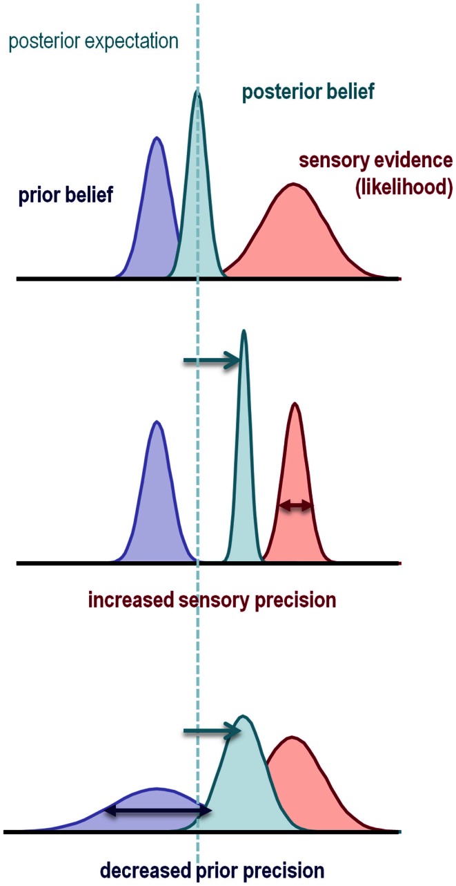
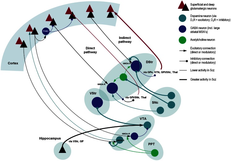
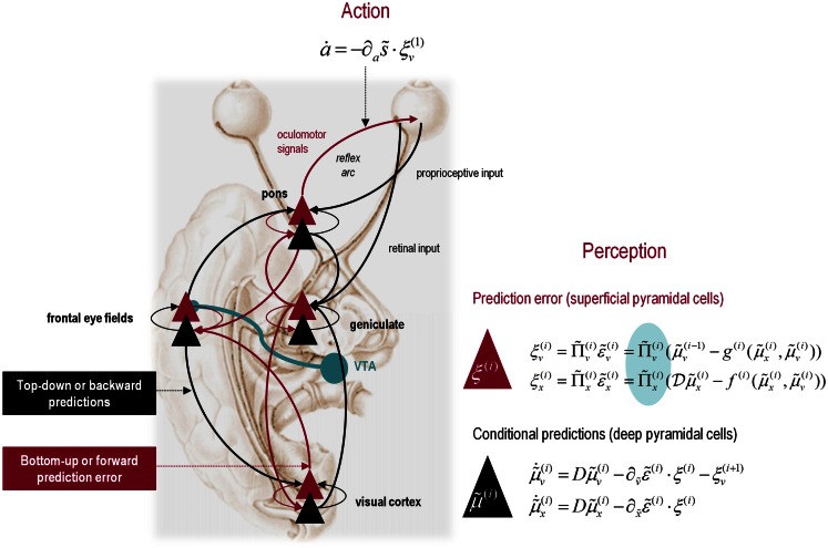
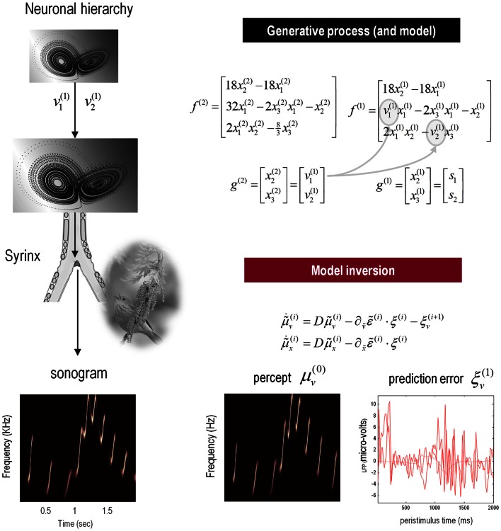
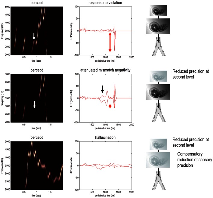
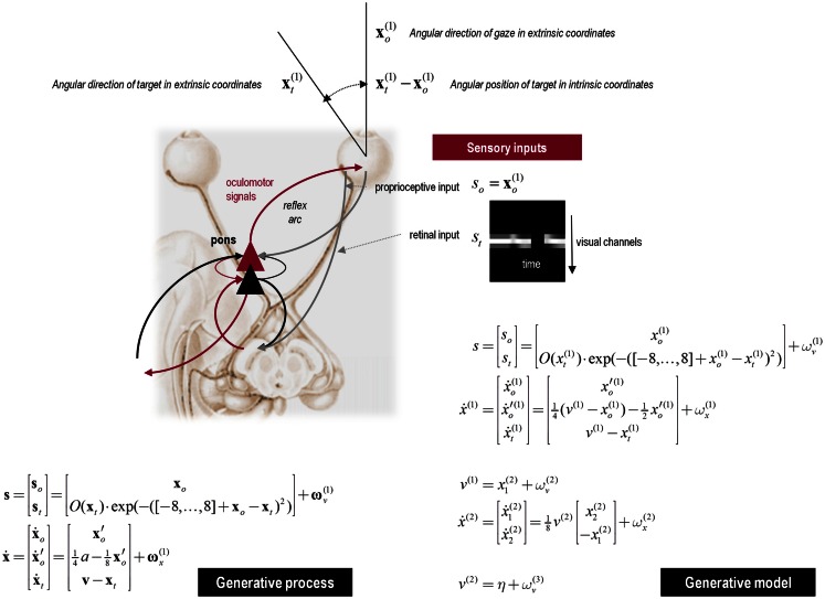
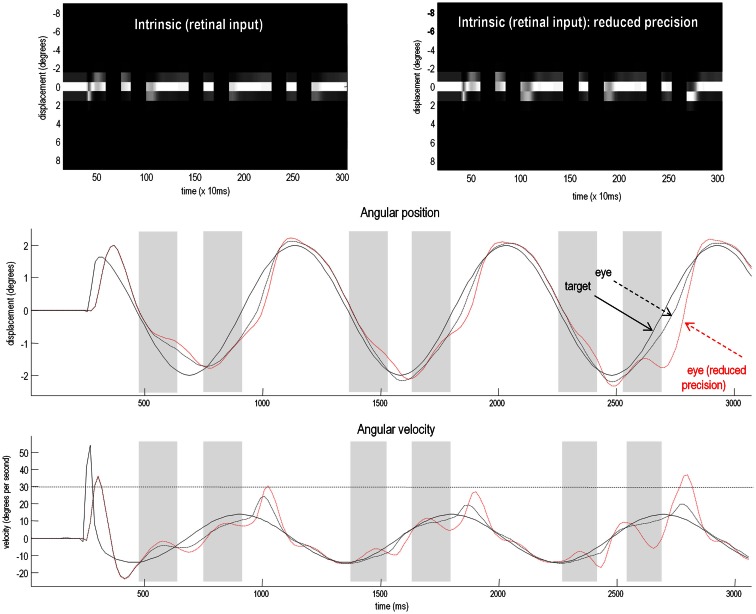
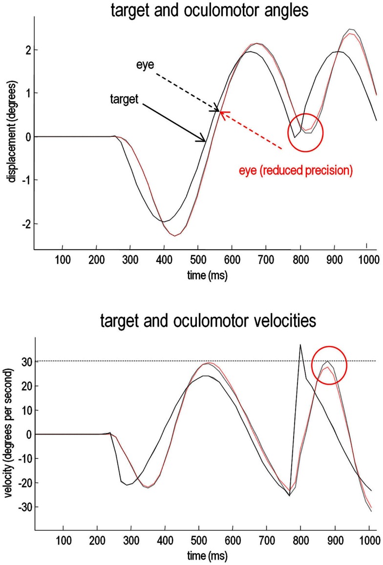
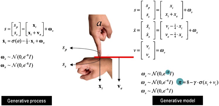
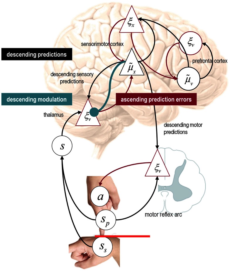
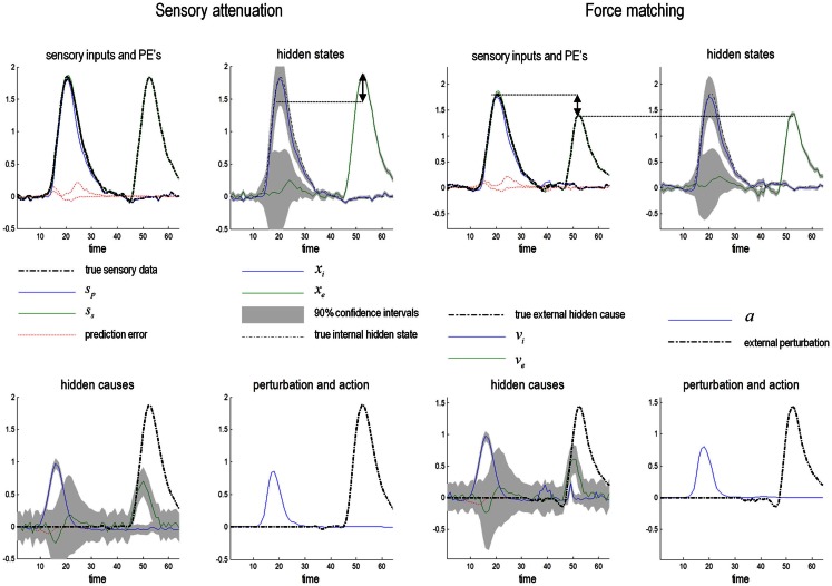
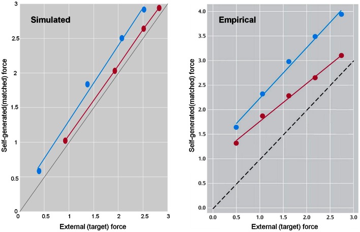
This paper considers psychotic symptoms in terms of false inferences or beliefs. It is based on the notion that the brain is an inference machine that actively constructs hypotheses to explain or predict its sensations. This perspective provides a normative (Bayes-optimal) account of action and perception that emphasizes probabilistic representations; in particular, the confidence or precision of beliefs about the world. We will consider hallucinosis, abnormal eye movements, sensory attenuation deficits, catatonia, and delusions as various expressions of the same core pathology: namely, an aberrant encoding of precision. From a cognitive perspective, this represents a pernicious failure of metacognition (beliefs about beliefs) that can confound perceptual inference. In the embodied setting of active (Bayesian) inference, it can lead to behaviors that are paradoxically more accurate than Bayes-optimal behavior. Crucially, this normative account is accompanied by a neuronally plausible process theory based upon hierarchical predictive coding. In predictive coding, precision is thought to be encoded by the post-synaptic gain of neurons reporting prediction error. This suggests that both pervasive trait abnormalities and florid failures of inference in the psychotic state can be linked to factors controlling post-synaptic gain - such as NMDA receptor function and (dopaminergic) neuromodulation. We illustrate these points using biologically plausible simulations of perceptual synthesis, smooth pursuit eye movements and attribution of agency - that all use the same predictive coding scheme and pathology: namely, a reduction in the precision of prior beliefs, relative to sensory evidence.

Keywords: active inference; free energy; illusions; precision; psychosis; schizophrenia; sensory attenuation.

Figure 1

This schematic illustrates the importance of precision when forming posterior beliefs and expectations. The graphs show Gaussian probability distributions that represent prior beliefs, posterior beliefs, and the likelihood of some data or sensory evidence as functions of some hidden (unknown) parameter. The dotted line corresponds to the posterior expectation, while the width of the distributions corresponds to their dispersion or variance. Precision is the inverse of this dispersion and can have a profound effect on posterior beliefs. Put simply, the posterior belief is biased toward the prior or sensory evidence in proportion to their relative precision. This means that the posterior expectation can be biased toward sensory evidence by either increasing sensory precision – or failing to attenuate it – or by decreasing prior precision.

Figure 2

A schematic illustration of putative pathological processes in schizophrenia – emphasizing the interactions among neuromodulatory mechanisms. These mechanisms include: (i) decreased prefrontal NMDA-R function that may reduce the stimulation of VTA-DA neurons that project back to prefrontal D₁Rs (decreasing cortical precision), and disinhibition of VTA-DA neurons that project to the striatum; (ii) increased dopamine release from SNc-DA neurons disinhibits the indirect pathway (by direct inhibition of striatal GABA neurons, inhibition of striatal cholinergic interneurons, and reduction of glutamate release in corticostriatal neurons); (iii) reduced NMDA-R stimulation of cortical PVBC’s reduces activity of these GABAergic interneurons, impairing coordination of cortical oscillatory activity; and (iv) increased hippocampal drive to the VTA, leading to hyperdopaminergia in the VStr. Significant omissions (for clarity) include: the GP, SNr, STN, and Thal, most connections of the VStr including its direct and indirect pathways and excitatory connections from the VTA (via D₁Rs), and circuitry within the VStr, two more inhibitory connections in the indirect pathway and both somatic and axonal dopamine neuron D₂ autoreceptors in SNc. As in other figures, descending projections are in black and ascending projections in red. Abbreviations: PPT, pedunculopontine tegmental nucleus; VTA, ventral tegmental area; VStr, ventral striatum; DStr, dorsal striatum; SNc/r, substantia nigra pars compacta/reticulata; GP, globus pallidus; Thal, thalamus; STN, subthalamic nucleus; PVBC, parvalbumin-positive basket cell. Stephan et al. (2009), Morrison (2012), Carlsson et al. (1999), Lisman et al. (2008), Simpson et al. (2010).

Figure 3

Hierarchical message passing in the visual-oculomotor system: the schematic illustrates a neuronal message-passing scheme (generalized Bayesian filtering or predictive coding) that optimizes posterior expectations about hidden states of the world, given sensory (visual) data, and the active (oculomotor) sampling of those data. It shows the speculative cells of origin of forward driving connections (in red) that convey prediction errors from a lower area to a higher area and the backward connections (in black) that construct predictions. These predictions try to explain away prediction error in lower levels. In this scheme, the sources of forward and backward connections are superficial (red) and deep (black) pyramidal cells respectively. The cyan connection denotes a neuromodulatory connection from the ventral tegmental area (VTA) which mediates estimates of precision. The equations on the right represent a generalized descent on free energy under the hierarchical model described in the main text – this can be regarded as a generalization of predictive coding or Bayesian (e.g., Kalman–Bucy) filtering. These equations are simplified versions of Eq. 3, in which state-dependent precision has been suppressed. State units are in black and error units are in red. The cyan circle highlights where precisions enter these equations – to modulate prediction error units (superficial pyramidal cells) such that they report precision-weighted prediction errors. In this schematic, we have placed different levels of a hierarchical model within the visual-oculomotor system. Visual input arrives in an intrinsic (retinal) frame of reference that depends on the direction of gaze. Exteroceptive input is then passed to the lateral geniculate nuclei (LGN) and to higher visual and prefrontal (e.g., frontal eye fields) areas in the form of prediction errors. Crucially, proprioceptive sensations are also predicted, creating prediction errors at the level of the cranial nerve nuclei (pons). The special aspect of these proprioceptive prediction errors is that they can be resolved in one of two ways: top-down predictions can change or the errors can be resolved through classical reflex arcs – in other words, they can elicit action to change the direction of gaze and close the visual–oculomotor loop.

Figure 4

Schematic showing the construction of the generative model for birdsongs. This comprises two Lorenz attractors where the higher attractor delivers two control parameters (gray circles in the corresponding equations of motion) to a lower level attractor, which, in turn, delivers two control parameters to a synthetic syrinx to produce amplitude and frequency modulated stimuli. These control parameters correspond to hidden causes that have to be inferred, given the stimulus. This stimulus is represented as a sonogram (lower left panel). The upper equations represent the hierarchical dynamic model in the form of Eq. 2; while the lower equations summarize the recognition or Bayesian filtering scheme in the form of (a simplified version of) Eq. 3. The lower right panels show the sensory predictions of this Bayesian filtering scheme in terms of the predicted sonogram based upon posterior expectations (left) and the precision-weighted prediction errors driving these expectations (right).

Figure 5

Omission-related responses. Here, we omitted the last three chirps from the stimulus. The left-hand panels show the predicted sonograms based upon posterior expectations, while the right-hand panels show the associated (precision weighted) prediction error at the sensory level. The top panels show a normal omission-related response using log precisions of 16 at the second (higher) level. This response is due to precise top-down predictions that are violated when the first missing chirp is not heard. This response is attenuated, when the log precision of the second level is reduced to two (middle row). This renders top-down predictions more sensitive to bottom-up sensory evidence and sensory prediction errors are resolved under reduced top-down constraints. At the same time, the third chirp – that would have been predicted on the basis of top-down (empirical) prior beliefs – is missed, leading to sensory prediction errors that nearly match the amplitude of the prediction errors elicited by the omission. The lower row shows predictions and prediction errors when there is a compensatory decrease in sensory log precision from two to minus two. Here, there is a failure of sensory prediction errors to entrain high-level expectations and subsequent false inference that persists in the absence of any stimuli.

Figure 6

Upper panel: this schematic summarizes the generative model for smooth pursuit eye movements. The model is based upon the prior belief that the center of gaze and target are attracted to a common (fictive) attracting point in visual space. The process generating sensory inputs is much simpler and is summarized by the equations specifying the generative process (lower left). The real-world provides sensory input in two modalities: proprioceptive input from cranial nerve nuclei reports the (horizontal) angular displacement of the eye s_o and corresponds to the center of gaze in extrinsic coordinates x_o. Exteroceptive (retinal) input reports the angular position of a target in a retinal (intrinsic) frame of reference s_t. This input models the response of 17 visual channels, each equipped with a Gaussian receptive field deployed at intervals of one angular unit – about 2° of visual angle. This input can be occluded by a function of target location O(x_t), which returns values between zero and one, such that whenever the target location x_t is behind the occluder retinal input is zero. The response of each visual channel depends upon the distance of the target from the center of gaze. This is just the difference between the oculomotor angle and target location. The hidden states of this model comprise the oculomotor states – oculomotor angle and velocity $\left({\text{x}}_o,\text{x}{\prime }_o\right)$ and the target location. Oculomotor velocity is driven by action and decays to zero with a time constant of eight time bins or 8 × 16 = 128 ms. This means the action applies forces to the oculomotor plant, which responds with a degree of viscosity. The target location is perturbed by the hidden cause v that describes the location to which the target is drawn (a sinusoid), with a time constant of one time bin or 16 ms. The random fluctuations on sensory input and the motion of hidden states had a log precision of 16. The generative model (lower right) has a similar form to the generative process but with two important exceptions: there is no action and the motion of the hidden oculomotor states is driven by the same hidden cause that moves the target. In other words, the agent believes that its gaze is attracted to the same fictive point in visual space that is attracting the target. Second, the generative model is equipped with a deeper (hierarchical) structure that can represent periodic trajectories in the hidden cause of target motion: hidden causes are informed by the dynamics of hidden states at a second level ${\dot{x}}^{(2)}$. These model sinusoidal fluctuations of any amplitude and a frequency – that is determined by a second level hidden cause v⁽²⁾ with a prior expectation of η. This prior expectation corresponds to beliefs about the frequency of periodic motion. The log precisions on the random fluctuations in the generative model were three at the first (sensory) level and minus one at the higher level, unless stated otherwise.

Figure 7

Smooth pursuit of a partially occluded target with and without high-level precision. These simulations show the results of applying Bayesian filtering Eq. 3 using the generative process and model of the previous figure. Notice, that in these simulations of active inference, there is no need to specify any stimuli explicitly – active sampling of the visual field means that the subject creates their own sensory inputs. The upper panels shows the responses of each of the (17) photoreceptors in image format as a function of peristimulus time. They illustrate the small fluctuations in signal that are due to imperfect pursuit and consequent retinal slip at the onset of target motion. Later, during periods of occlusion, the sensory input disappears. The lower panels show the angular displacement (top) and velocity (bottom) of the target (solid lines) and eye (broken lines) as a function of peristimulus time. They illustrate the remarkably accurate tracking behavior that is produced by prior beliefs that the center of gaze and target are drawn to the same fictive point – beliefs that action fulfils. The gray area corresponds to the period of visual occlusion. The upper right panel shows sensory input when the precision of prediction errors on the motion of hidden states at the second level was reduced from a log precision of −1 to −1.25. The associated behavior is shown with red broken lines in the lower panels. The dashed horizontal line in the lower panel corresponds to an angular velocity (30°); at which the eye movement would be considered saccadic. This simulation illustrates the loss of Bayes-optimal tracking when the motion of the target corresponds to high-level posterior beliefs but the precision of these beliefs is attenuated.

Figure 8

Smooth pursuit with an unexpected trajectory change – with and without high-level precision: this figure reports the simulations of occluded periodic motion with a reversal in the direction of the trajectory at the beginning of the second cycle (plain black line). The broken traces in black correspond to normal pursuit and the broken traces in red show the performance under reduced precision. Although the effect is small, reducing the precision about prior beliefs produces more accurate pursuit performance, both in terms of the displacement between the target and center of gaze and in terms of a slight reduction in the peak velocity during the compensatory eye movement (red circles). This illustrates the paradoxical improvement of performance that rest upon precise sensory information that cannot be predicted a priori (and is characteristic of syndromes like schizophrenia and autism).

Figure 9

This figure shows the generative process and model used in the simulations of sensory attenuation. The generative process (on the left) models real-world states and causes, while the model on the right is the generative model used by the subject. In the real world, the hidden state x_i corresponds to self-generated pressures that are sensed by both somatosensory s_s and proprioceptive s_p input channels. External forces are modeled with the hidden cause v_e and are sensed only by the somatosensory channel. Action causes the self-generated force x_i to increase and is modified by a sigmoid squashing function σ. The hidden state decays slowly over four time bins. In the generative model, causes of sensory data are divided into internal v_i and external causes v_e. The hidden cause excites dynamics in hidden states x_i and x_e, which decay slowly. Internal force is perceived by both proprioceptive and somatosensory receptors, as before, while external force is perceived only by somatosensory receptors. Crucially, the precision of the sensory input ω_s is influenced by the level of internal force, again modulated by a squashing function, and controlled by a parameter γ that governs the level of attenuation of precision. The generalized predictive coding scheme associated with this generative model is shown schematically in the next figure.

Figure 10

Speculative mapping of Eq. 3 – for the generative model in the previous figure – onto neuroanatomy. Somatosensory and proprioceptive prediction errors are generated by the thalamus, while the expectations and prediction errors about hidden states (the forces) are placed in sensorimotor cortex. The expectations and prediction errors about the hidden causes of forces have been placed in the prefrontal cortex. Under active inference, proprioceptive predictions descend to the spinal cord and elicit output from alpha motor neurons (playing the role of proprioceptive prediction error units) via a classical reflex arc. Red connections originate from prediction error units – ξ cells – and can be regarded as intrinsic connections or ascending (forward) extrinsic connections (from superficial pyramidal cells). Conversely, the black connections represent intrinsic connections and descending (backward) efferents (from deep pyramidal cells) encoding posterior expectations – $\tilde{\mu }$ cells. The cyan connection denotes descending neuromodulatory effects that mediate sensory attenuation. The crucial point to take from this schematic is that conditional expectations of sensory states (encoded in the pyramidal cell ${\tilde{\mu }}_x$) can either be fulfilled by descending proprioceptive predictions (that recruit classical reflex arcs) or they can be corrected by ascending sensory prediction errors. In order for descending motor efferents to prevail, the precision of the sensory prediction errors must be attenuated.

Figure 11

Simulation of the force-matching task. The x axes denote time in 100 ms time bins; the y axes force in Newtons. Left panels: in the first part of this simulation an internal force is generated from a prior belief about the cause v_i, followed by the presentation of an external force. Posterior beliefs about the hidden states (upper right panel) are similar, but the confidence interval around the force for the internally generated state is much broader. This is because sensory level precision must be attenuated in order to allow proprioceptive predictions to be fulfilled by reflex arcs instead of being corrected by sensory input: i.e., the confidence intervals around v_i must be narrower than those around x_i to allow movement to proceed. If perceived intensity of the sensation is associated with the lower 90% confidence bound of the estimate of hidden state (highlighted by the dotted line), it will be lower when the force is self generated than when the force is exogenous (the difference is highlighted by the arrow). Right panels: the simulation was repeated but the external force was matched to the lower bound of the 90% confidence interval of the internal force. This means that internally generated force is now greater than the externally applied force (double-headed arrow, upper left panel). This reproduces the normal psychophysics of the force-matching illusion that can be regarded as entirely Bayes-optimal, under appropriate levels of precision.

Figure 12

Left panel: the force-matching simulation was repeated under different levels of self-generated force. For normal levels of sensory attenuation (blue circles), internally produced force is higher than externally generated force at all levels. Data from patients with schizophrenia was simulated by attenuating sensory precision and increasing the precision of prediction errors at higher levels of the hierarchy. This resulted in a more veridical perception of internally generated force (red circles). Right panel: the empirical data from the force-matching task, with normal subjects’ forces in blue, and schizophrenics’ forces in red reproduced from Shergill et al. (2005).

Figure 13

Pathology of sensory attenuation. Left panel: here sensory attenuation is much lower (γ = 2). In this case, bottom-up prediction errors have a higher precision than top-down predictions: the confidence intervals around v_i (bottom left panel) are now broader than those around x_i (upper right panel). The expected hidden state is thus profoundly suppressed (upper right panel), meaning proprioceptive prediction errors are not produced (upper left panel) and action is suppressed (lower right panel) resulting in akinesia. Right panels: to simulate the force-matching results seen in schizophrenia, precision at the second level of the hierarchy was increased to allow movement. The underlying failure of sensory attenuation still enables a precise and accurate perception of internally and externally generated sensations (upper left panel). However, the causes of sensory data are not accurately inferred: a false (delusional) cause (lower left panel) is perceived during internally generated movement that is antagonistic to the movement. This is because the proprioceptive prediction errors driving action are rendered overly precise, meaning higher levels of the hierarchy must be harnessed to explain them, resulting in a delusion that exogenous forces are opposing the expected outcome (encircled in red).

References

1. Abi-Saab W. M., D’Souza D. C., Moghaddam B., Krystal J. H. (1998). The NMDA antagonist model for schizophrenia: promise and pitfalls. Pharmacopsychiatry 31 (Suppl. 2), 104–10910.1055/s-2007-979354 - DOI - PubMed
1. Adams R. A., Perrinet L. U., Friston K. (2012). Smooth pursuit and visual occlusion: active inference and oculomotor control in schizophrenia. PLoS ONE 7:e47502.10.1371/journal.pone.0047502 - DOI - PMC - PubMed
1. Adams R. A., Shipp S., Friston K. J. (2013). Predictions not commands: active inference in the motor system. Brain Struct. Funct. 218, 611–64310.1007/s00429-012-0475-5 - DOI - PMC - PubMed
1. Albrecht M. A., Martin-Iverson M. T., Price G., Lee J., Iyyalol R., Waters F. (2011). Dexamphetamine effects on separate constructs in the rubber hand illusion test. Psychopharmacology (Berl.) 217, 39–5010.1007/s00213-011-2255-y - DOI - PubMed
1. Allen P., Aleman A., McGuire P. K. (2007). Inner speech models of auditory verbal hallucinations: evidence from behavioural and neuroimaging studies. Int. Rev. Psychiatry 19, 407–41510.1080/09540260701486498 - DOI - PubMed
LinkOut - more resources