Adaptive stimulus optimization for sensory systems neuroscience

Abstract

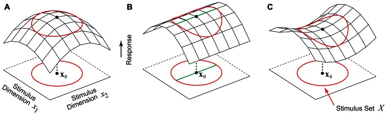
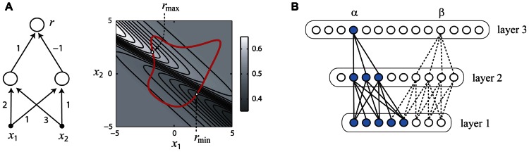
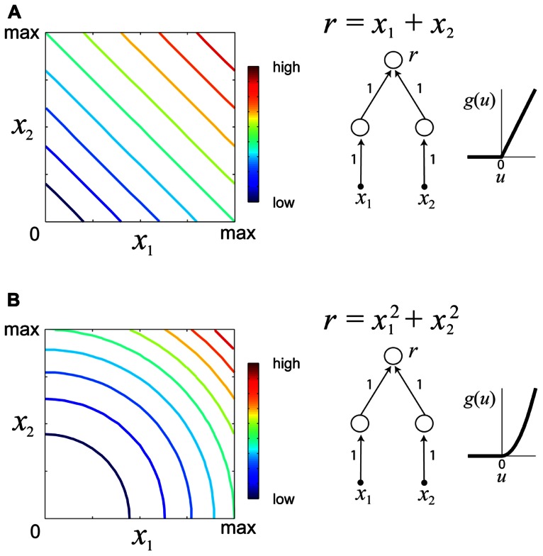
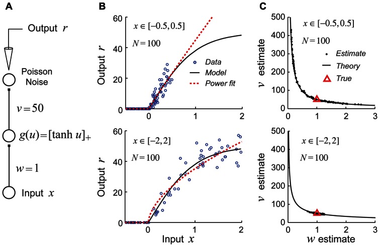
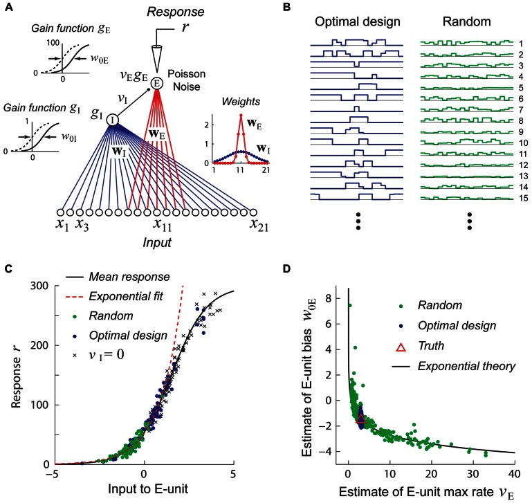
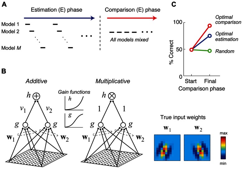
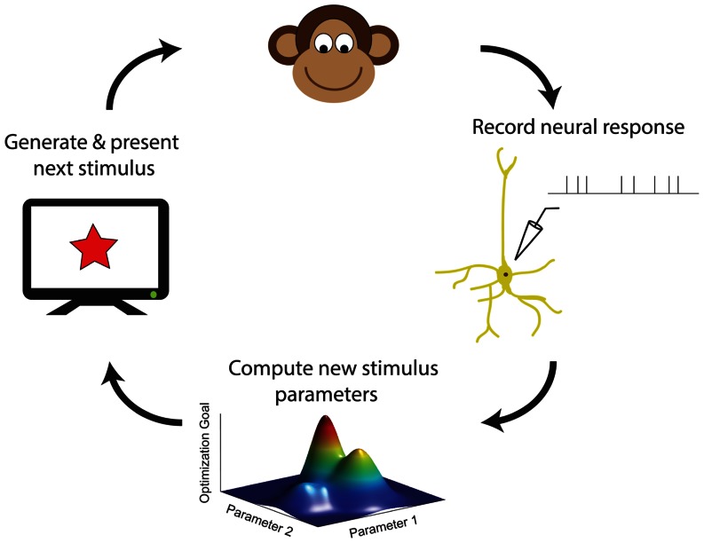
In this paper, we review several lines of recent work aimed at developing practical methods for adaptive on-line stimulus generation for sensory neurophysiology. We consider various experimental paradigms where on-line stimulus optimization is utilized, including the classical optimal stimulus paradigm where the goal of experiments is to identify a stimulus which maximizes neural responses, the iso-response paradigm which finds sets of stimuli giving rise to constant responses, and the system identification paradigm where the experimental goal is to estimate and possibly compare sensory processing models. We discuss various theoretical and practical aspects of adaptive firing rate optimization, including optimization with stimulus space constraints, firing rate adaptation, and possible network constraints on the optimal stimulus. We consider the problem of system identification, and show how accurate estimation of non-linear models can be highly dependent on the stimulus set used to probe the network. We suggest that optimizing stimuli for accurate model estimation may make it possible to successfully identify non-linear models which are otherwise intractable, and summarize several recent studies of this type. Finally, we present a two-stage stimulus design procedure which combines the dual goals of model estimation and model comparison and may be especially useful for system identification experiments where the appropriate model is unknown beforehand. We propose that fast, on-line stimulus optimization enabled by increasing computer power can make it practical to move sensory neuroscience away from a descriptive paradigm and toward a new paradigm of real-time model estimation and comparison.

Keywords: adaptive data collection; neural network; optimal stimulus; parameter estimation; sensory coding.

FIGURE 1

Hypothetical stimulus–response relationships for a sensory neuron. The red circle represents the boundary of the set of permissible stimuli. (A) Stimulus x₀ is a firing rate peak which corresponds to the intuitive notion of the optimal stimulus where any perturbation away from x₀ results in a decrease in the firing rate. (B) This neuron is tuned to one stimulus dimension but is insensitive to the second dimension. Instead of a single optimal stimulus x₀ there is a continuum of optimal stimuli (green line). (C) A neuron whose stimulus–response function around the point x₀ is saddle-shaped. Along one stimulus dimension x₀ is a firing rate maximum, and along the other stimulus dimension x₀ is a minimum.

FIGURE 2

How the optimal stimulus properties of sensory neurons may be constrained by network architecture. Panels (A,B) adapted with permission from DiMattina and Zhang (2008). (A) A simple neural network (left) and its responses to inputs x₁, x₂ (right). The optimal stimulus for this network must lie on the boundary of any closed set of stimuli (right panel, thick red line). (B) The functional network connecting a single neuron (α or β) to the sensory periphery may have fewer units in successive processing layers (convergent), even if the overall number of neurons in successive processing layers is increasing (divergent).

FIGURE 3

Examples of iso-responses surfaces for two hypothetical sensory processing models. (A) Iso-response contours (left) of a sensory neuron which linearly integrates stimulus variables x₁, x₂ ≥ 0. The response r of this neuron is a summation of the outputs of two neurons in the lower layer with a threshold-linear gain function (right). Colors in the contour plot represent neural firing rates from low to high. (B) Iso-responses contours (right) of a sensory neuron which non-linearly integrates stimulus variables x₁, x₂ ≥ 0 with a threshold-quadratic gain function (right).

FIGURE 4

Example of continuous parameter confounding in a simple non-linear neural network model. Adapted with permission from DiMattina and Zhang (2010). (A) A simple three layer neural network whose input and output weight parameters (w,v) we wish to estimate from noisy stimulus–response data. Noise is drawn from a Poisson distribution. (B) Top: The input stimuli x ∈ [-0.5, 0.5] only drive the hidden unit over a limited region of its gain function (black curve) which may be well approximated by a power law function (red dashed line). Bottom: The input stimuli x ∈ [-2,2] drive the hidden unit over a larger region of its gain function which is poorly approximated by a power law function. (C) Top: When trained with sets of stimuli like that in the top of Figure 4B, the estimates (black dots) lie scattered along the curve predicted by the power law confounding theory. Bottom: When trained with sets of stimuli like those in the bottom panel of Figure 4B, the true parameter values (red triangle) are more reliably recovered.

FIGURE 5

Stimuli which are adaptively optimized for accurate parameter estimation can be more effective than random stimuli for recovering non-linear models. Adapted with permission from DiMattina and Zhang (2011). (A) A simple center-surround neural network consisting of a narrowly integrating excitatory output unit (E-unit) which receives inhibitory input from a broadly integrating interneuron (I-unit). (B) Examples of optimally designed (left) and random (right) stimuli. Note that the optimally designed stimuli exhibit complex correlated structure. (C) Random stimuli (green dots) only drive the E-unit over a limited range of its gain function (black curve) which may be well approximated by an exponential function (red dashed line). This is due to inhibition from the I-unit, as can be seen by setting v_I = 0 (crosses). By contrast, optimally designed stimuli (blue dots) drive the gain function over its full range. (D) Estimates attained from training with random stimuli (green dots) exhibit continuous parameter confounding between the output weight and bias, as predicted by the exponential theory (black curve). In contrast, estimates attained from optimally designed stimuli accurately recover the true parameters (red triangle).

FIGURE 6

Stimuli which are adaptively optimized for model comparison can lead to more accurate model selection. Adapted with permission from DiMattina and Zhang (2011). (A) A hypothetical two phase procedure for estimating and comparing multiple competing models. During the estimation (E) phase, stimuli are optimized in turn for estimating each model. During the comparison (C) phase, stimuli are optimized for comparing all of the models. (B) Two candidate models were fit to data generated by a true additive model whose input weights (w₁ and w₂) were 12 × 12 Gabor patches shown at the right. The two competing models differ only in their method of integrating subunit activities (additive versus multiplicative). (C) At the end of the estimation phase (“Start”), the BIC does not consistently prefer either model. Presenting additional stimuli optimized for model discrimination yields almost perfect model selection (red curve), while presenting additional random stimuli (green curve), or stimuli optimized for model estimation (blue curve) either does not improve or only somewhat improves model selection.

FIGURE 7

A schematic summary of closed-loop approaches in sensory neurophysiology. Neural responses to previous stimuli are used in order to choose new stimuli, by maximizing an objective function for accomplishing a desired experimental goal (see also Table 1).

References

1. Ahmadian Y., Packer A. M., Yuste R., Paninski L. (2011). Designing optimal stimuli to control neuronal spike timing. J. Neurophysiol. 106 1038–1053 - PMC - PubMed
1. Ahrens M. B., Linden J. F., Sahani M. (2008a). Nonlinearities and contextual influences in auditory cortical responses modeled with multilinear spectrotemporal methods. J. Neurosci. 28 1929–1942 - PMC - PubMed
1. Ahrens M. B., Paninski L., Sahani M. (2008b). Inferring input nonlinearities in neural encoding models. Network 19 35–67 - PubMed
1. Albrecht D. G., DeValois R. L., Thorell L. G. (1980). Visual cortical neurons: are bars or gratings the optimal stimuli? Science 207 88–90 - PubMed
1. Albrecht D. G., Hamilton D. B. (1982). Striate cortex of monkey and cat: contrast response function. J Neurophysiol. 48 217–237 - PubMed
Publication types