

Chaos and reliability in balanced spiking networks with temporal drive
- PMID: 23767592
- PMCID: PMC4124755
- DOI: 10.1103/PhysRevE.87.052901
Chaos and reliability in balanced spiking networks with temporal drive
Abstract
Biological information processing is often carried out by complex networks of interconnected dynamical units. A basic question about such networks is that of reliability: If the same signal is presented many times with the network in different initial states, will the system entrain to the signal in a repeatable way? Reliability is of particular interest in neuroscience, where large, complex networks of excitatory and inhibitory cells are ubiquitous. These networks are known to autonomously produce strongly chaotic dynamics-an obvious threat to reliability. Here, we show that such chaos persists in the presence of weak and strong stimuli, but that even in the presence of chaos, intermittent periods of highly reliable spiking often coexist with unreliable activity. We elucidate the local dynamical mechanisms involved in this intermittent reliability, and investigate the relationship between this phenomenon and certain time-dependent attractors arising from the dynamics. A conclusion is that chaotic dynamics do not have to be an obstacle to precise spike responses, a fact with implications for signal coding in large networks.
Figures


 . For all panels except A (top), network parameters: η = −0.5, ε = 0.5 with λ1 ≈ 2.5.
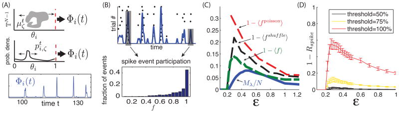


Similar articles
-
Encoding in Balanced Networks: Revisiting Spike Patterns and Chaos in Stimulus-Driven Systems.PLoS Comput Biol. 2016 Dec 14;12(12):e1005258. doi: 10.1371/journal.pcbi.1005258. eCollection 2016 Dec. PLoS Comput Biol. 2016. PMID: 27973557 Free PMC article.
-
Balanced state of networks of winner-take-all units.PLoS Comput Biol. 2025 Jun 11;21(6):e1013081. doi: 10.1371/journal.pcbi.1013081. eCollection 2025 Jun. PLoS Comput Biol. 2025. PMID: 40498862 Free PMC article.
-
Experimental study of firing death in a network of chaotic FitzHugh-Nagumo neurons.Phys Rev E Stat Nonlin Soft Matter Phys. 2013 Feb;87(2):022919. doi: 10.1103/PhysRevE.87.022919. Epub 2013 Feb 28. Phys Rev E Stat Nonlin Soft Matter Phys. 2013. PMID: 23496603
-
Overview of facts and issues about neural coding by spikes.J Physiol Paris. 2010 Jan-Mar;104(1-2):5-18. doi: 10.1016/j.jphysparis.2009.11.002. Epub 2009 Nov 29. J Physiol Paris. 2010. PMID: 19925865 Review.
-
A spiking neural network architecture for nonlinear function approximation.Neural Netw. 2001 Jul-Sep;14(6-7):933-9. doi: 10.1016/s0893-6080(01)00080-6. Neural Netw. 2001. PMID: 11665783 Review.
Cited by
-
Nonlinear stimulus representations in neural circuits with approximate excitatory-inhibitory balance.PLoS Comput Biol. 2020 Sep 18;16(9):e1008192. doi: 10.1371/journal.pcbi.1008192. eCollection 2020 Sep. PLoS Comput Biol. 2020. PMID: 32946433 Free PMC article.
-
Driving reservoir models with oscillations: a solution to the extreme structural sensitivity of chaotic networks.J Comput Neurosci. 2016 Dec;41(3):305-322. doi: 10.1007/s10827-016-0619-3. Epub 2016 Sep 2. J Comput Neurosci. 2016. PMID: 27585661
-
Structured chaos shapes spike-response noise entropy in balanced neural networks.Front Comput Neurosci. 2014 Oct 2;8:123. doi: 10.3389/fncom.2014.00123. eCollection 2014. Front Comput Neurosci. 2014. PMID: 25324772 Free PMC article.
-
Encoding in Balanced Networks: Revisiting Spike Patterns and Chaos in Stimulus-Driven Systems.PLoS Comput Biol. 2016 Dec 14;12(12):e1005258. doi: 10.1371/journal.pcbi.1005258. eCollection 2016 Dec. PLoS Comput Biol. 2016. PMID: 27973557 Free PMC article.
-
Sensory Stream Adaptation in Chaotic Networks.Sci Rep. 2017 Dec 4;7(1):16844. doi: 10.1038/s41598-017-16478-z. Sci Rep. 2017. PMID: 29203867 Free PMC article.
References
-
- Eigen M, Gardiner W, Schuster P, Winkleroswatitsch R. Scientific american. 1981;244 - PubMed
-
- Bialek W, Rieke F, de Ruyter Van Steveninck R, Warland D. Science. 1991;252:1854. - PubMed
-
- Uchida A, McAllister R, Roy R. Physical review letters. 2004;93 - PubMed
-
- Rulkov N, Sushchik M, Tsimring L, Abarbanel H. Physical Review E. 1995 Jan;51:980. - PubMed
-
- Lin K, Shea-Brown E, Young LS. J Nonlin Sci. 2009;19(5):497.
Publication types
MeSH terms
Grants and funding
LinkOut - more resources
Full Text Sources
Other Literature Sources