The Virtual Brain: a simulator of primate brain network dynamics

Abstract

We present The Virtual Brain (TVB), a neuroinformatics platform for full brain network simulations using biologically realistic connectivity. This simulation environment enables the model-based inference of neurophysiological mechanisms across different brain scales that underlie the generation of macroscopic neuroimaging signals including functional MRI (fMRI), EEG and MEG. Researchers from different backgrounds can benefit from an integrative software platform including a supporting framework for data management (generation, organization, storage, integration and sharing) and a simulation core written in Python. TVB allows the reproduction and evaluation of personalized configurations of the brain by using individual subject data. This personalization facilitates an exploration of the consequences of pathological changes in the system, permitting to investigate potential ways to counteract such unfavorable processes. The architecture of TVB supports interaction with MATLAB packages, for example, the well known Brain Connectivity Toolbox. TVB can be used in a client-server configuration, such that it can be remotely accessed through the Internet thanks to its web-based HTML5, JS, and WebGL graphical user interface. TVB is also accessible as a standalone cross-platform Python library and application, and users can interact with the scientific core through the scripting interface IDLE, enabling easy modeling, development and debugging of the scientific kernel. This second interface makes TVB extensible by combining it with other libraries and modules developed by the Python scientific community. In this article, we describe the theoretical background and foundations that led to the development of TVB, the architecture and features of its major software components as well as potential neuroscience applications.

Keywords: connectome; full-brain network model; large-scale simulation; neural masses; python; time delays; virtual brain; web platform.

Figure 1

The Virtual Brain Architecture: TVB provides two independent interfaces depending on the interaction with users. Blocks in the back-end are transparently used by different top application layers. TVB-Datatypes, are the common language between different components (analyzers, visualizers, simulator, uploaders). They represent “active data” in the sense that, when TVB is configured with a database, data contained in TVB-Datatypes instances are automatically persistent. Currently the console interface works without the storage layer, keeping the results just in memory. S-Users need to manually handle data import and export operations.

Figure 2

Main working areas of The Virtual Brain 's web interface: in USER personal information (account settings) as well as hardware and software preferences (technical settings) are configured. Through the PROJECT area users access and organize their projects, data, figures and the operations dashboard. Input and output simulated data can be exported in HDF5 format and may be used outside of the framework. Brain network models and execution of simulations are configured and launched, respectively in SIMULATOR. In this area results can be immediately analyzed and visualized to have a quick overview of the current model. A history of launched simulations is kept to have the traceability of any modifications that took place in the simulation chain. STIMULUS provides a collection of tools to build stimulation patterns that will be available to use in the simulations. Finally, CONNECTIVITY provides an interactive environment to the edit and visualize connectivity matrices.

Figure 3

UI screenshots. (A) SIMULATOR Area. Having multiple panels allows a quick overview of previous simulations (left), model parameters for the currently selected simulation (middle), and summary displays of the data associated with the currently selected simulation (right). (B) Shows the interface for editing and visualising the structural connectivity, for one of the six possible connectivity visualisations. (C) PROJECT Area—operations dashboard. On the left column, users can compose filters to search through all the operations on the list.

Figure 4

Demonstration datasets exist in TVB for the anatomical structure on which simulations are built, including a triangular mesh surface representation of the neocortex (A) and white matter fiber lengths (B). However, new data from structural imaging such as MRI, DTI, and DSI for individual subjects, as well as data from the literature can be used and wrapped in a TVB-Datatype.

Figure 5

Diagram of the configurable elements for building a brain network model and launching a simulation. TVB can incorporate cortical connectivity information from an individual's tractographic and cortical geometry data. The Connectivity object contains matrices defining the connection strengths and time delays via finite signal transmission speed between all regions, while the folded Cortical Surface mesh provides the spatial support for finer resolution models. In the latter case a Local Coupling defines the interaction between neighboring nodes. In its simplest form local connectivity is spatially invariant, however, support exists for spatial inhomogeneity. Signal propagation via local connectivity is instantaneous (no time delays), which is a reasonable approximation considering the short distances involved. Together, the cortical surface with its local connectivity, the long-range connectivity matrix, and the neural mass models defining the local dynamics define a full brain network model. Additionally, stimulation can be applied to a simulation. The stimulation patterns are built in terms of spatial and temporal equations chosen independently. For region-based network models, it is only possible to build time dependent stimuli since there is not a spatial extent for a region node. However, node-specific weightings can be set to modulate the intensity of the stimulus applied to each node. For surface-based models, equations with finite spatial support are evaluated as a function of distance from one or more focal points (vertices of the surface), where the equation defines the spatial profile of the stimuli. The neural source activity from both region or surface-based approaches can be projected into EEG, MEG and BOLD (Buxton and Frank, ; Friston et al., 2000) space using a forward model (Breakspear and Jirsa, 2007).

Figure 6

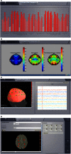
Visualizers. (A) Histogram of a graph metric as a function of nodes in the connectivity matrix. (B) A 2D projection of the head. The color map represents a graph metric computed on the connectivity matrix. (C) EEG visualizer combines a rendered head surface, an overlay with the sensors positions and an interactive time-series display. (D) An animated display of the spatiotemporal pattern applied to the cortical surface. Red spots represent the focal points of the spatial component of the stimulus.

Figure 7

(A) As expected for fixed time-step schemes, execution times scale linearly with the number of integration steps. We used seven values of simulation lengths (1, 2, 4, 8, 16, 32, and 64 s) and five values of integration time step (dt = 2⁻² = 0.25, dt = 2⁻³ = 0.125, dt = 0.0625 = 2⁻⁴, dt = 0.03125 = 2⁻⁵, and dt = 0.015625 = 2⁻⁶ ms). For each possible combination 100 simulations were performed. The network model consisted of 74 nodes (with two state variables and one mode per node). Numerical integration was based on Heun's stochastic method. We plot the average execution time with the error bars representing the standard deviation over simulations. The inset shows a narrower range for simulation lengths between 1 and 4 s. Axes units and color code are the same as those displayed in the main plot. (B) Here, execution times are shown as a function of the integration time step size, dt, for two different number of nodes (solid and dashed lines correspond to connectivity matrices of 64 and 128 nodes, respectively) for a specific conduction speed (4 mm/ms) and simulation length (64 s). Both axes are in logarithmic scale with base 2. In this case, halving dt or doubling the number of nodes in the connectivity matrix, N, doubles the running time. However, as mentioned in the text, for larger networks execution times seem to grow quadratically as a function of the number of nodes in the network. Further tests need to be developed to understand this behavior.

Figure 8

Phase portrait using TVB's interactive phase plane tool (accessible from both shell and graphical interfaces): the blue line corresponds to a trajectory of a single oscillator node isolated and without noise, 4th order Runge-Kutta integration scheme. In the bottom panel, the corresponding trajectories of both the v(t) and w(t) state variables of the model are shown. The activity exhibits oscillations at approximately 40 Hz.

Figure 9

(A) The activity of individual regions are illustrated in colored lines. The black line represents the average activity over the network nodes. Here brain regions are weakly coupled changing both the collective and local dynamics of the network. (B) Using TVB scientific library as a python module we can conveniently run thousands of simulations in parallel on a cluster. Note that TVB parallelizes different tasks e.g., simulations and analyses, taking advantage of multi-core systems, however, it does not parallelize the processes themselves. Simultaneous simulations allow for a systematic parameter space exploration to rapidly gain insights of the whole brain dynamics repertoire. In this plot, the magnitude and color scale correspond to one the variance computed over all the elements of the N-dimensional output array (Global Variance). Simulations were performed on a cluster based on the Python demo scripts available in the release packages. On of the major strengths of The Virtual Brain is that G-Users are enabled to launch parameter sweeps through the UI without the need to know how to submit parallel jobs (see Figure 10).

Figure 10

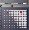
One of TVB's major strengths is the capability to launch parallel simulations through the UI. We show a screenshot of the resulting display when sweeping across two different parameters of the Generic2dOscillator model. Here each data point represents two metrics: size is mapping the Global Variance and color corresponds to the Variance of the nodes Variance. These results provide a topography of the stability space allowing users to distinguish, and thus select, combinations of critical parameters values.

Figure 11

(A) The upper left blue panel shows the raw traces of nodes V2 and V1; the latter stimulated with a rectangular pulse of width equal to 5 ms and repetition frequency of 1 Hz. Signals are normalized by their corresponding maximum value. The right blue panel show the signals for a shorter period of time. Amplitudes are not normalized to emphasize the relative difference between the two regions. Middle panels illustrate the stimulus pattern. Lower red panels display the activity as projected onto EEG space and recorded from channels Oz and O1. The default EEG cap in TVB consists of 62 scalp electrodes distributed according to the 10–20 international system (Klem et al., 1999). In this simulation a deterministic integration scheme was employed to obtain the time-series of neural activity, since noise was not applied to the model's equations. (B) The same description as in (A) applies. The main difference with the previous simulation is that here white noise was added to the system.

Figure 12

The green and blue panels show EEG recordings from electrode Oz during the resting state, i.e., in the absence of stimulation and in the stimulated condition, respectively, notice the slow damped oscillations after stimulus onset at a approximately 10 Hz; the light gray trace depicts the stimulation pattern. The bottom panel displays multiscale entropy estimates computed on the Oz time-series at different temporal scales using the dataset obtained by means of a stochastic integration scheme.

References

1. Amari S. (1975). Homogeneous nets of neuron-like elements. Biol. Cybern. 17, 211–220 10.1007/bf00339367 - DOI - PubMed
1. Amari S. (1977). Dynamics of pattern formation in lateral-inhibition type neural fields. Biol. Cybern. 22, 77–87 10.1007/BF00337259 - DOI - PubMed
1. Assisi C., Jirsa V., Kelso J. (2005). Synchrony and clustering in heterogeneous networks with global coupling and parameter dispersion. Phys. Rev. Lett. 94:018106 10.1103/PhysRevLett.94.018106 - DOI - PubMed
1. Atay F., Hutt A. (2006). Neural fields with distributed transmission speeds and long range feedback delays. SIAD 5, 670–698 10.1137/050629367 - DOI
1. Babajani-Feremi A., Soltanian-Zadeh H. (2010). Multi-area neural mass modeling of eeg and meg signals. Neuroimage 52, 793–811 10.1016/j.neuroimage.2010.01.034 - DOI - PubMed