New Python-based methods for data processing

Abstract

Current pixel-array detectors produce diffraction images at extreme data rates (of up to 2 TB h(-1)) that make severe demands on computational resources. New multiprocessing frameworks are required to achieve rapid data analysis, as it is important to be able to inspect the data quickly in order to guide the experiment in real time. By utilizing readily available web-serving tools that interact with the Python scripting language, it was possible to implement a high-throughput Bragg-spot analyzer (cctbx.spotfinder) that is presently in use at numerous synchrotron-radiation beamlines. Similarly, Python interoperability enabled the production of a new data-reduction package (cctbx.xfel) for serial femtosecond crystallography experiments at the Linac Coherent Light Source (LCLS). Future data-reduction efforts will need to focus on specialized problems such as the treatment of diffraction spots on interleaved lattices arising from multi-crystal specimens. In these challenging cases, accurate modeling of close-lying Bragg spots could benefit from the high-performance computing capabilities of graphics-processing units.

Keywords: cctbx; data processing; multiprocessing; reusable code.

Figure 1

Overall organization of cctbx, showing selected modules relevant to the applications described in this article. In addition to standalone core modules, cctbx provides object-oriented Python bindings to the C-­language libraries CMTZ (Winn et al., 2002 ▶), CBFlib (Bernstein & Ellis, 2005 ▶) and ANN (Arya et al., 1998 ▶). Python scripting allows the cctbx code to interoperate with externally developed packages. Functions of interest are provided by the packages NumPy (http://www.numpy.org), mod_python (Trubetskoy, 2007 ▶), pyana, wxPython (Rappin & Dunn, 2006 ▶), matplotlib (http://matplotlib.org), PyCUDA (Klöckner et al., 2012 ▶) and h5py (http://code.google.com/p/h5py).

Figure 2

Client–server architecture for a high-throughput Bragg spot analyzer. The illustrated client (a) is a web browser, but the client is usually the beamline component responsible for the raster scan, such as Blu-Ice (McPhillips et al., 2002 ▶) or GDA (Aishima et al., 2010 ▶), implemented in any language that supports the HTTP protocol. The server (b) is a multicore Linux system running the Apache httpd daemon, which delegates incoming requests to one of 48 parallel child processes, each of which runs Python-language cctbx code mediated by the mod_python package (c). The server returns text-based output identical to that produced by the command-line program distl.signal_strength. There is also an option for the returned text to be formatted in extensible markup language (XML) suitable for automated control-system clients. Full instructions are given at http://cci.lbl.gov/labelit/html/client_server.html.

Figure 3

Concurrent processing of femtosecond crystallography data at LCLS with cctbx.xfel. A file-mediated approach is taken in which the data-acquisition system multiplexes the detector images to several serial-access binary streams written in extended tagged container (XTC) format (a). For data analysis, each of the six XTC files is assigned to a separate 12-core Linux node, on which the pyana framework reads the data within a single master process and delegates the analysis of consecutive images to as many as 11 child processes. pyana provides a Python-language callback hook to be executed once for each image, into which is inserted the cctbx spotfinder code. As the XTC file is on a shared-disk file system, data acquisition and processing are performed simultaneously. Although processing lags behind acquisition for any given XTC file, the ‘run’ is switched after a few minutes to a new XTC file, so the overall processing throughput roughly keeps up. (b) Bragg spot counts/image are shown for a 70 min 483 845-image thermolysin data set (Sierra et al., 2012 ▶) broken into 12 runs starting at the indicated wall clock times. The hit rate (defined as the fraction of images with ≥16 Bragg spots within a defined area) is plotted over a 5 s sliding window. The total number of hits is 15 094.

Figure 4

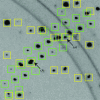
Indexing model from an exposure illuminating two lysozyme microcrystals collected at ALS beamline 5.0.1 using an ADSC Q315 detector. Most reflections on the two lattices (yellow and green) are well separated, but some come close enough to impinge on the integration box chosen for modeling spots on the other lattice (a), while a few overlap outright (b).

Figure 5

(a) Cross-platform wxPython-based phenix.image_viewer application included in cctbx. (b) Detail of the prototype cctbx.image_viewer, which exposes a programming interface for displaying models. Here, the red box and blue dot are alternate models of the Bragg diffraction recorded on a PAD detector; the models have not been optimized and thus differ substantially from the center position of the observed Bragg spot (green dot).

Figure 6

(a) Low-order fringe pattern for a photosystem I crystallite calculated on a GPU and similar to that actually observed at the LCLS (Chapman et al., 2011 ▶). (b) Computational efficiency of evaluating (1) scaling as N ² (number of atoms × number of structure factors). The CPU calculation was performed single-threaded on a 64-bit Intel Xeon (2.4 GHz), 8 MB cache, 23.5 GB RAM running Scientific Linux 5.4 with code compiled under GCC 4.4.2. GPU calculations were either on an Nvidia C1060 (Tesla, 1.30 GHz), 4.0 GB on-device memory, 960 hardware cores or on the higher-performance Nvidia C2050 (Fermi, 1.15 GHz), 2.6 GB on-device memory, 448 hardware cores; both were programmed in CUDA. The top plot (blue crosses) depicts calculations run with 32-bit (single) precision; otherwise, calculations were in 64-bit (double) precision. A comparison is given with the FFT method, which scales as NlogN. The loss of accuracy observed on moving from 64-bit to 32-bit precision is generally less than the loss of accuracy (typically 0.8%) resulting from use of the FFT approximation rather than (1). Example code is available at http://cctbx.svn.sourceforge.net/viewvc/cctbx/trunk/cctbx/x-ray/structure_factors/from_scatterers_direct_parallel.py. Python bindings for CUDA utilize the PyCUDA package (Klöckner et al., 2012 ▶). Benchmarks in (b) are performed on a single unit cell in space group P1, while the simulation in (a) is over all atoms in 10 × 12 × 14 unit cells in space group P6₃. Simulation (a) scales as N ² as it uses (1).

References

1. Abrahams, D. & Grosse-Kunstleve, R. W. (2003). C/C++ Users J. 21, 29–36.
1. Adams, P. D. et al. (2010). Acta Cryst. D66, 213–221. - PubMed
1. Aishima, J., Owen, R. L., Axford, D., Shepherd, E., Winter, G., Levik, K., Gibbons, P., Ashton, A. & Evans, G. (2010). Acta Cryst. D66, 1032–1035. - PMC - PubMed
1. Arya, S., Mount, D. M., Netanyahu, N. S., Silverman, R. & Wu, A. Y. (1998). J. Assoc. Comput. Mach. 45, 891–923.
1. Barty, A. et al. (2012). Nature Photonics 6, 35–40. - PMC - PubMed
Publication types