Life as we know it

Abstract

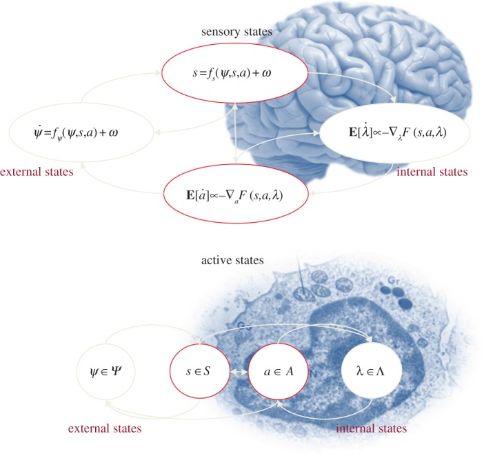
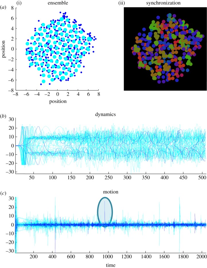
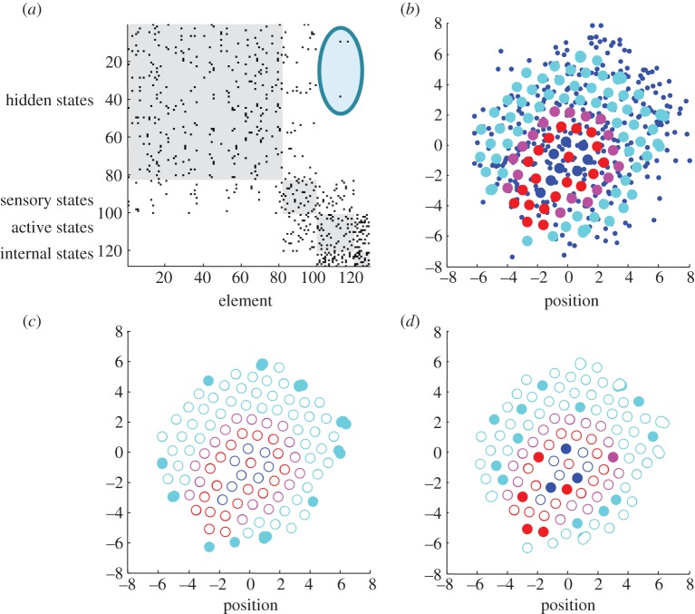
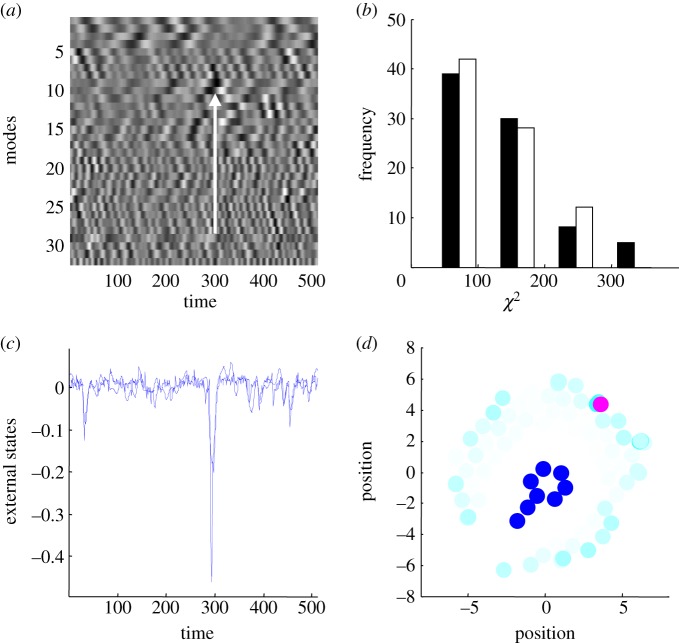
This paper presents a heuristic proof (and simulations of a primordial soup) suggesting that life-or biological self-organization-is an inevitable and emergent property of any (ergodic) random dynamical system that possesses a Markov blanket. This conclusion is based on the following arguments: if the coupling among an ensemble of dynamical systems is mediated by short-range forces, then the states of remote systems must be conditionally independent. These independencies induce a Markov blanket that separates internal and external states in a statistical sense. The existence of a Markov blanket means that internal states will appear to minimize a free energy functional of the states of their Markov blanket. Crucially, this is the same quantity that is optimized in Bayesian inference. Therefore, the internal states (and their blanket) will appear to engage in active Bayesian inference. In other words, they will appear to model-and act on-their world to preserve their functional and structural integrity, leading to homoeostasis and a simple form of autopoiesis.

Keywords: active inference; autopoiesis; ergodicity; free energy; random attractor; self-organization.

Figure 1.

Markov blankets and the free energy principle. These schematics illustrate the partition of states into internal states and hidden or external states that are separated by a Markov blanket—comprising sensory and active states. The upper panel shows this partition as it would be applied to action and perception in the brain; where—in accord with the free energy principle—active and internal states minimize a free energy functional of sensory states. The ensuing self-organization of internal states then corresponds to perception, while action couples brain states back to external states. The lower panel shows exactly the same dependencies but rearranged so that the internal states can the associated with the intracellular states of a cell, while the sensory states become the surface states or cell membrane overlying active states (e.g. the actin filaments of the cytoskeleton). See table 1 for a definition of variables.

Figure 2.

Ensemble dynamics. (a) The position of (128) subsystems comprising an ensemble after 2048 s. a(i) The dynamical status (three blue dots per subsystem) of each subsystem centred on its location (larger cyan dots). a(ii) The same information, where the relative values of the three dynamical states of each subsystem are colour-coded (using a softmax function of the three functional states and a RGB mapping). This illustrates the synchronization of dynamical states within each subsystem and the dispersion of the phases of the Lorenzian dynamics over subsystems. (b,c) The evolution of functional  and structural states as a function of time, respectively. The (electrochemical) dynamics of the internal (blue) and external (cyan) states are shown for the 512 s. One can see initial (chaotic) transients that resolve fairly quickly, with itinerant behaviour as they approach their attracting set. (c) The position of internal (blue) and external (cyan) subsystems over the entire simulation period illustrate critical events (circled) that occur every few hundred seconds, especially at the beginning of the simulation. These events generally reflect a pair of particles (subsystems) being expelled from the ensemble to the periphery, when they become sufficiently close to engage short-range repulsive forces. These simulations integrated the stochastic differential equations in the main text using a forward Euler method with 1/512 s time steps and random fluctuations of unit variance.

Figure 3.

Emergence of the Markov blanket. (a) The adjacency matrix that indicates a conditional dependency (spatial proximity) on at least one occasion over the last 256 s of the simulation. The adjacency matrix has been reordered to show the partition of hidden (cyan), sensory (magenta), active (red) and internal (blue) subsystems, whose positions are shown in (b)—using the same format as in the previous figure. Note the absence of direct connections (edges) between external or hidden and internal subsystem states. The circled area illustrates coupling between active and hidden states that are not reciprocated (there are no edges between hidden and active states). The spatial self-organization in the upper left panel is self evident; where the internal states have arranged themselves in a small loop structure with a little cilium, protected by the active states that support the surface or sensory states. When viewed as a movie, the entire ensemble pulsates in a chaotic but structured fashion, with the most marked motion in the periphery. (c,d) Highlights those subsystems that cannot influence others (closed subsystems (c)) and those that have slower dynamics (slow subsystems (d)). The remarkable thing here is that all the closed subsystems have been rusticated to the periphery—where they provide a locus for vigorous dynamics and motion. Contrast this with the deployment of slow subsystems that are found throughout the hidden, sensory, active and internal partition.

Figure 4.

Self-organized perception. This figure illustrates the Bayesian perspective on self-organized dynamics. (a) The first (principal) 32 eigenvariates of the internal (functional) states as a function of time over the last 512 s of the simulations reported in the previous figures. These eigenvariates were obtained by a singular value decomposition of the timeseries over all internal functional states (lagged between plus and minus 16 s). These represent a summary of internal dynamics that are distributed over internal subsystems. The eigenvariates were then used to predict the (two-dimensional) motion of each external subsystem using a standard canonical variates analysis. The (classical) significance of this prediction was assessed using Wilks' lambda (following a standard transformation to the χ² statistic). The actual (dotted line) and predicted (solid line) position for the most significant external subsystem is shown in (c)—in terms of canonical variates (best linear mixture of position in two dimensions). The agreement is self-evident and is largely subtended by negative excursions, notably at 300 s. The fluctuations in internal states are visible in (a) and provide a linear mixture that correlates with the external fluctuation (highlighted with a white arrow). The location of the external subsystem that was best predicted is shown by the magenta circle on (d). Remarkably, this is the subsystem that is the furthest away from the internal states and is one of the subsystems that participates in the exchanges a closed subsystem in the previous figure. (c) Also shows the significance with which the motion of the remaining external states could be predicted (with the intensity of the cyan being proportional to the χ² statistic above). Interestingly, the motion that is predicted with the greatest significance is restricted to the periphery of the ensemble, where the external subsystems have the greatest latitude for movement. To ensure this inferential coupling was not a chance phenomenon, we repeated the analysis after flipping the external states in time. This destroys any statistical coupling between the internal and external states but preserves the correlation structure of fluctuations within either subset. The distribution of the ensuing χ² statistics (over 82 external elements) is shown in (b) for the true (black) and null (white) analyses. Crucially, five of the subsystems in the true analysis exceeded the largest statistic in the null analysis. The largest value of the null distribution provides protection against false positives at a level of 1/82. The probability of obtaining five χ² values above this threshold by chance is vanishingly small p = 0.00052.

Figure 5.

Autopoiesis and oscillator death. These results show the trajectory of the subsystems for 512 s after the last time point characterized in the previous figures. (a) The trajectories under the normal state of affairs; showing a preserved and quasicrystalline arrangement of the internal states (blue) and the Markov blanket (active states in red and sensory states in magenta). Contrast this formal self-organization with the decay and dispersion that ensues when the internal states and Markov blankets are synthetically lesioned (b,c,d). In all simulations, a subset of states was lesioned by simply rendering their subsystems closed—in other words, although the Newtonian interactions were preserved, they were unable to affect the functional states of neighbouring subsystems. (b) The effect of this relatively subtle lesion on active states—that are rapidly expelled from the interior of the ensemble, allowing sensory states to invade and disrupt the internal states. A similar phenomenon is seen when the sensory states were lesioned (c)—as they drift out into the external system. There is a catastrophic loss of structural integrity when the internal states themselves cannot affect each other, with a rapid migration of internal states through and beyond their Markov blanket (d). These simulations illustrate the effective death of biological self-organization that is a well-known phenomenon in dynamical systems theory—known as oscillator death: see [58]. In our setting, they are a testament to autopoiesis or self-creation—in the sense that self-organized dynamics are necessary to maintain structural or configurational integrity.

References

1. Schrödinger E. 1944. What is life?: the physical aspect of the living cell. Dublin, Ireland: Trinity College.
1. Ashby WR. 1947. Principles of the self-organizing dynamic system. J. Gen. Psychol. 37, 125–128. (10.1080/00221309.1947.9918144) - DOI - PubMed
1. Haken H. 1983. Synergetics: an introduction. Non-equilibrium phase transition and self-selforganisation in physics, chemistry and biology, 3rd edn Berlin, Germany: Springer.
1. Maturana HR, Varela F. (eds) 1980. Autopoiesis and cognition. Dordrecht, The Netherlands: Reidel.
1. Nicolis G, Prigogine I. 1977. Self-organization in non-equilibrium systems. New York, NY: Wiley.
Publication types
MeSH terms
LinkOut - more resources