Deformable M-Reps for 3D Medical Image Segmentation

Abstract

M-reps (formerly called DSLs) are a multiscale medial means for modeling and rendering 3D solid geometry. They are particularly well suited to model anatomic objects and in particular to capture prior geometric information effectively in deformable models segmentation approaches. The representation is based on figural models, which define objects at coarse scale by a hierarchy of figures - each figure generally a slab representing a solid region and its boundary simultaneously. This paper focuses on the use of single figure models to segment objects of relatively simple structure. A single figure is a sheet of medial atoms, which is interpolated from the model formed by a net, i.e., a mesh or chain, of medial atoms (hence the name m-reps), each atom modeling a solid region via not only a position and a width but also a local figural frame giving figural directions and an object angle between opposing, corresponding positions on the boundary implied by the m-rep. The special capability of an m-rep is to provide spatial and orientational correspondence between an object in two different states of deformation. This ability is central to effective measurement of both geometric typicality and geometry to image match, the two terms of the objective function optimized in segmentation by deformable models. The other ability of m-reps central to effective segmentation is their ability to support segmentation at multiple levels of scale, with successively finer precision. Objects modeled by single figures are segmented first by a similarity transform augmented by object elongation, then by adjustment of each medial atom, and finally by displacing a dense sampling of the m-rep implied boundary. While these models and approaches also exist in 2D, we focus on 3D objects. The segmentation of the kidney from CT and the hippocampus from MRI serve as the major examples in this paper. The accuracy of segmentation as compared to manual, slice-by-slice segmentation is reported.

Fig. 1

A 2D illustration of (left) the traditional view of the medial locus of an object as a sheet of disks (spheres in 3D) bitangent to the object boundary and our equivalent view (right) as an m-rep: a curve (sheet in 3D) of hubs at the sphere center and equal length spokes normal to object boundary. The locus of the spoke ends forms the medially implied boundary.

Fig. 2

M-reps: In the 2D example (left) there are 4 figures: a main figure, a protrusion, an indentation, and a separate object. Each figure is represented by a chain of medial atoms. Certain medial atoms in a subfigure are interfigurally linked (dashed lines on the left) to their parent figures. In the 3D example of a hippocampus (middle) there is one figure, represented by a mesh of medial atoms. Each hub with two line segment spokes forms a medial atom (Fig. 3). The mesh is viewed from two directions, and the renderings below show the boundary implied by the mesh. The example on the right shows a 4-figure m-rep for a cerebral ventricle.

Fig. 3

Medial atoms, made from a position x and two equal length boundary-pointing arrows p⃗ and s⃗ (for “port” and “starboard”), which we call “spokes”. The atom on the left is for an internal mesh position, implying two boundary sections. The atom on the right is for a mesh edge position, implying a section of boundary crest. The atoms are shown in the “atom-plane” containing x, p⃗ and s⃗. An atom is represented by the medial hub position x; the length r of the boundary-pointing arrows; a frame made from the unit-length bisector b⃗ of p⃗ and s⃗, the b⃗ - orthogonal unit vector n⃗ in the atom plane, and the complementary unit vector b⃗^⊥; and the “object angle” θ between b⃗ and each spoke. For a slab-like section of figure, p⃗ and s⃗ provide links between the medial point and the implied boundary (shown as a narrow curve), giving approximations, with tolerance, to both its position and its normal. The implied figure section is slab-like and centered on the head of the atom's spokes, i.e., it is extended in the b⃗^⊥ direction just as it is illustrated to do in the atom-plane directions perpendicular to its spoke.

Fig. 4

Left: A single-figure m-rep. Left middle: Coarse mesh of atom boundary positions for a figure. Right middle: Atom ends vs. interpolated boundary. Right: interpolated boundary mesh at voxel spacing

Fig. 5. Correspondence over deformation via figural correspondence

Fig. 6

M-reps models. Heavy dots show hubs of medial atoms. Lines are atoms' spokes. The mesh connecting the medial atoms is shown as dotted curves. Implied boundaries are rendered with shading. Hippocampus: see Fig. 2. Left: kidney parenchyma + renal pelvis. Middle: lateral horn of cerebral ventricle. Right: multiple single-figure objects in male pelvis: rectum, prostate, bladder, and pubic bones (one bone is occluded in this view).

Fig. 7

The viewing planes of interest for a medial atom: Top: 3D views. Bottom: 2D views.

Fig. 8

The collar forming the mask for measuring geometry to image match. Left: in 2D, both before and after deformation. Right: in 3D, showing the boundary as a mesh and showing three cross-sections of the collar.

Fig. 9

Segmentation results of the lateral horn of a cerebral ventricle at the m-rep level of scale (i.e., before boundary displacement) from MRI using a single figure model.

Fig. 10

Sagittal plane through a CT of the kidney, used in this study, demonstrating significant partial volume and breathing artifacts. A human segmentation is shown as a green tint. Note the scalloped boundary and spurious sections of the kidney, which were segmented by one of two human raters but excluded by m-rep segmentation. Note also the nearby high-contrast rib that can create a repulsive force when a Gaussian derivative template is used.

Fig. 11

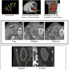
Stage by stage progress: all rows, from left to right, show results on Coronal, Sagittal and Axial CT slices. Each row compares progress through consecutive stages via overlaid grey curves to show the kidney segmentation after stage N vs. white curves after stage N+1. Top row: stages are the initial position of the kidney model vs. the figural similarity transform plus elongation. Middle: the similarity transform plus elongation vs. medial atom transformations. Bottom: medial atom transformations vs. 3D boundary displacements.

Fig. 12

Kidney model and segmentation results. Segmentation results at the m-rep level of scale (i.e., before boundary displacement) on kidneys in CT using a single figure model. The three light curves on the rendered m-rep implied boundary in the 3D view above right show the location of the slices shown in the center row. On these slices the curve shows the intersection of the m-rep implied boundary with the slices. The slices in the lower row are the sagittal and coronal slices shown in the 3D view.

Fig. 13. Scattergram of median surface separations for all kidneys

Figure 14

Valmet pairwise comparisons for a left kidney. The comparison result is color-coded on a reference surface selected from human (A or B) and m-rep segmentations (see Fig. 15). Green represents a subvoxel surface correspondence between the two compared segmentations. Red represents a section where the surface of the reference segmentation is outside the compared surface. Blue represents a section where the surface of the reference segmentation is inside compared surface. Left: Reference shape from human B, color coding from human A. Middle: Reference shape from human B, color coding from m-reps. Right: Reference shape from m-reps, color coding from human B. In this case the volume overlap for A and B was 93.5% and the m-rep overlap was 94.0% with both A and B.

Figure 15

Valmet comparisons for a kidney with significant motion artifacts (see Fig. 10), reflecting human segmentations' preservation of artifactual scalloping vs. the m-rep segmentations' yielding a smooth surface. Left: Reference shape from human A, color coding from human B. In this case both A and B contoured spurious sections at the top of the kidney, but rater A contoured one additional slice. Center: Reference shape from m-reps, color coding from human A. Right: Color coding scheme.

Fig. 16

Correctable m-rep failure mistakenly included in our analysis (worst case in Table 1). Left: Valmet comparison with reference shape from human B, color coding from m-reps. Center: Sagittal plane showing m-rep (blue) and human (red) surfaces. Two problems mentioned in the text are illustrated. In the region labeled “A” the m-rep model deformed into structures related to the kidney pelvis that were poorly differentiated from the kidney parenchyma. In the region labeled “B” the m-rep model did not elongate fully during the first transformation stage. Right: Transverse plane illustrating the deformation of the m-rep model into peri-pelvic structures in region A. Even in this case there is close correspondence between human and m-rep contours excluding regions A and B. After more careful user-guided initialization a successful m-rep segmentation was obtained for this kidney, but those results were omitted in the analysis.

Fig. 17

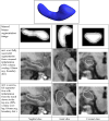
Hippocampus results using training intensity matches, for one of the three target images with typical results. The top image shows the m-rep-segmented hippocampus from the blurred binary segmentation image. Each row in the table shows in three intersecting triorthogonal planes the target image overlaid with the implied boundary of the m-rep hippocampus segmentation using the image template match. The top row shows the segmentation from the blurred binary image produced from a human segmentation. The middle row shows the corresponding segmentation using the mri image as the target and an intialization from a manual placement of the model determined from training image. The bottom row shows the segmentation of the same target mri with both the initialization and the model being the segmentation result on the blurred binary image for that case.

References

1. Amenta N, Bern M, Kamvysselis M. A New Voronoi-Based Surface Reconstruction Algorithm. Computer Graphics; Proceedings, Annual Conference Series; 1998; ACM SIGGRAPH; 1998. pp. 415–422.
1. Attali D, Sanniti di Baja G, Thiel E. Skeleton simplification through non significant branch removal. Image Processing and Communications. 1997;3(3-4):63–72.
1. Bittar E, Tsingos N, Gascuel M. Automatic Reconstruction of Unstructured 3D Data: Combining a Medial Axis and Implicit Surfaces. Computer Graphics Forum (Eurographics '95) 1995;14(3):457–468.
1. Blum H. A transformation for extracting new descriptors of shape. In: Wathen-Dunn W, editor. Models for the Perception of Speech and Visual Form. MIT Press; Cambridge MA: 1967. pp. 363–380.
1. Burbeck CA, Pizer SM, Morse BS, Ariely D, Zauberman G, Rolland J. Linking object boundaries at scale: a common mechanism for size and shape judgments. University of North Carolina Computer Science Department technical report TR94-041. Vision Research. 1996;36(3):361–372. - PubMed