. 2013 Aug 7;58(15):5173-92.
doi: 10.1088/0031-9155/58/15/5173. Epub 2013 Jul 9.

Bladder wall thickness mapping for magnetic resonance cystography

Affiliations

Bladder wall thickness mapping for magnetic resonance cystography

Yang Zhao et al. Phys Med Biol. .

Abstract

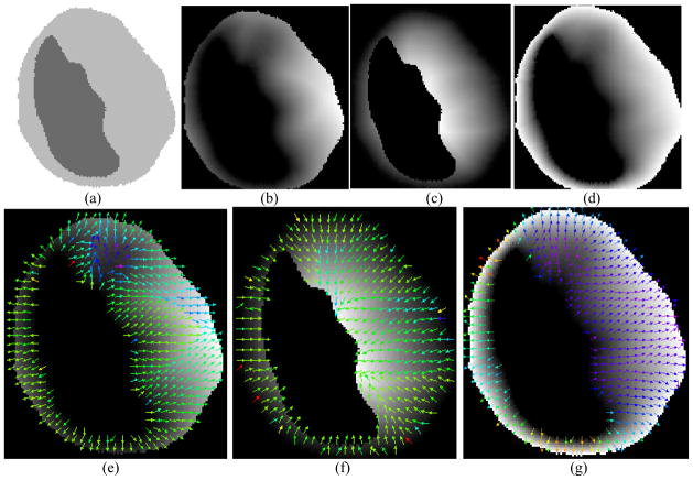
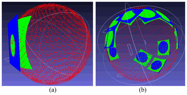
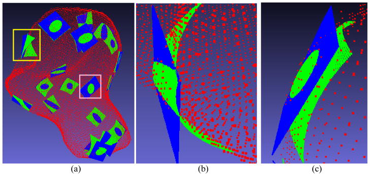
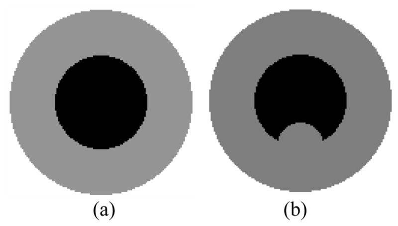
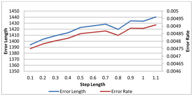
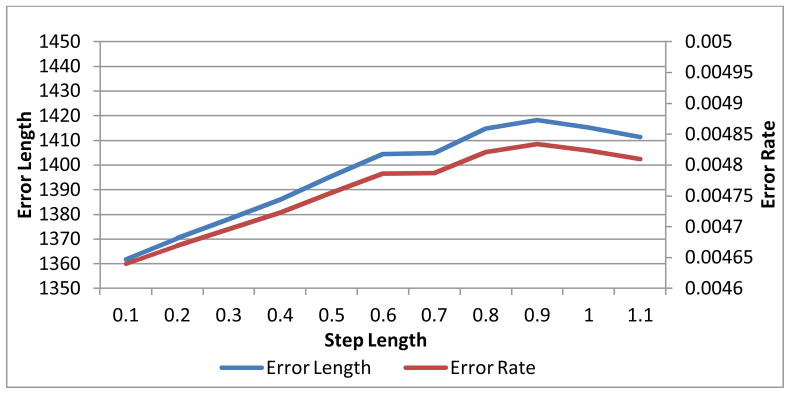
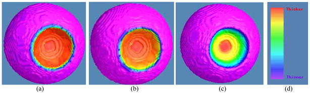
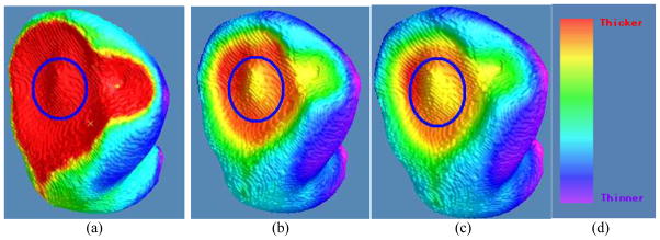
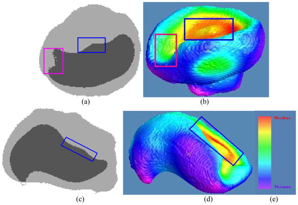
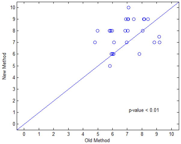
Clinical studies have shown evidence that the bladder wall thickness is an effective biomarker for bladder abnormalities. Clinical optical cystoscopy, the current gold standard, cannot show the wall thickness. The use of ultrasound by experts may generate some local thickness information, but the information is limited in field-of-view and is user dependent. Recent advances in magnetic resonance (MR) imaging technologies lead MR-based virtual cystoscopy or MR cystography toward a potential alternative to map the wall thickness for the entire bladder. From a high-resolution structural MR volumetric image of the abdomen, a reasonable segmentation of the inner and outer borders of the bladder wall can be achievable. Starting from here, this paper reviews the limitation of a previous distance field-based approach of measuring the thickness between the two borders and then provides a solution to overcome the limitation by an electric field-based strategy. In addition, this paper further investigates a surface-fitting strategy to minimize the discretization errors on the voxel-like borders and facilitate the thickness mapping on the three-dimensional patient-specific bladder model. The presented thickness calculation and mapping were tested on both phantom and human subject datasets. The results are preliminary but very promising with a noticeable improvement over the previous distance field-based approach.


Figures

Fig. 1
Fig. 1
The thick curves represent the ideal inner and the outer borders. The dashed curves represent the iso-distance surfaces computed by the DT-based method between the two ideal borders. The thin curves indicate the paths from one border to the other. (a) It shows a path traced in the DT field built based on the inner border (higher curve). (b) It shows the same local shape of the bladder walls, but the DT field is built based on the outer border (lower curve). The path traced here differs from that in (a). (c) The “tumor” has a hemisphere shape. By the DT-based method, the thicknesses at A, B, C are calculated as along AOP¯,BOP¯,COP¯ respectively, which are the same and do not reflect the true thickness changes. (d) The paths starting from A, B, C are computed by the electric-field line tracing method and have different lengths, i.e., the paths in (d) are more sensitive than that in (c) and more reasonable.
Fig. 2
Fig. 2
A particular case for the present method.
Fig. 3
Fig. 3
(a) A slice of the segmented bladder area of a patient dataset. (b) Distance field computed based on inner wall. The grey value of the image shows the distance from inner wall: the larger the grey value is the larger the distance is. (c) Distance field computed based on the outer wall. (d) Distance field computed based on both inner and outer walls. (e), (f) and (g) The sampled gradient directions used to trace paths in the distance field corresponding to (b), (c), and (d), respectively.
Fig. 4
Fig. 4
One slice from the middle of the phantom with one surface embedded. The border voxels are marked as value 2 and the other parts are all marked as 0.
Fig. 5
Fig. 5
(a) The approximating surface obtained by the MLS method around the voxel at (23, 21, 5). Each voxel is corresponding to a red point. The blue plane is the fitted hyperplane (from the step 1 in Section 2.4) and the green one shows the fitted quadratic surface (from the step 2 in Section 2.4). (b) More samples at 10 random selected positions.
Fig. 6
Fig. 6
(a) An overview of 20 local approximating surfaces on a patient study. (b) A closer view of the local approximating surface marked by the yellow rectangle in (a). (c) A closer view of the local surface marked by the pink rectangle in (a).
Fig. 7
Fig. 7
Two-dimensional presentations of normal and abnormal bladder wall models. (a) – Normal case where the phantom was made as a sphere. (b) – Abnormal case where the phantom was made as a sphere plus a “tumor” part at the bottom of inner border.
Fig. 8
Fig. 8
The errors v.s. the step length of the experiment without the MLS surface fitting.
Fig. 9
Fig. 9
The errors v.s. the step length of the experiment with the MLS surface fitting.
Fig. 10
Fig. 10
Thickness mappings on the 3D bladder phantom model with abnormality using the three methods of (a) the previous DT-based method [17], (b) the presented DT-based method in Section 2.2, and (c) the presented EFLT method in Section 2.3. Picture (d) shows the color bar for the thickness values over the phantom, where the red end indicates a higher value (thicker) while the purple end indicates a smaller value (thinner).
Fig. 11
Fig. 11
Thickness mappings on the 3D patient bladder, where the colors are superimposed on the inner surface mesh, by the three methods of (a) the previous DT-based method [17], (b) the presented DT-based method in Section 2.2, and (c) the presented EFLT method in Section 2.3. Note that the circled parts on the three pictures demonstrate that (b) and (c) have a much higher sensitivity to show the variation of the thickness around the tumor than (a), and furthermore (c) is some more sensitive than (b). (d) The same color bar as used in Fig. 10.
Fig. 12
Fig. 12
Demonstration of the consistency between the original segmented data and the visualization of the thickness mapping in Fig. 11. Picture (a) shows a section of an image slice along the X-Z plane. The boundary of the darker part is the bladder wall inner border. Picture (b) is the generated 3D view of the bladder wall inner border as shown in the pose corresponding to (a). Note that the regions marked by blue rectangles on both (a) and (b) indicate the same region as shown in Fig. 11(b). They together demonstrate the consistency: a small bump in a large basin. This consistency can also be observed by the region marked by the pink rectangles in both (a) and (b). By rotating the image volumes to another orientation for an image slice of (c) along the Y-Z plane, the generated 3D view of the bladder wall inner border is then shown by (d) in the pose corresponding to (c). The regions marked by blue rectangles in (c) and (d) indicate the same region as the one marked in (a), (b) and Fig. 11(b). This further demonstrates the consistency among them. (e) is the color bar same as used in Fig. 10 and 11.
Fig. 13
Fig. 13
Scatter plot of experts’ scores on both thickness calculation methods. The horizontal axis represents the score of the DT-based method and the vertical axis represents the score of the EFLT method. Each point represents a pair of scores for both methods. The scatter plot used a Jitter plot technique, which allows multiple observations with the same plotted values to be observable on the plot by adding a small amount of random noises to the values [27].
Fig. 14
Fig. 14
The thickness distribution of the patient dataset of Fig. 10.

Similar articles

Cited by

References

    1. Siegel R, Naishadham D, Jemal A. Cancer statistics, 2013. A Cancer Journal for Clinicians. 2013;63:11–30. - PubMed
    1. Shaw ST, Poon SY, Wong ET. Routine urinalysis: Is the dipstick enough? The Journal of the American Medical Association. 1985;253:1596–1600. - PubMed
    1. Grossfeld GD, Carroll PR. Evaluation of asymptomatic microscopic hematuria. Urologic Clinics of North America. 1998;25:661–676. - PubMed
    1. Sievert K, Amend B, Nagele U, Schilling D, Bedke J, Horstmann M, Hennenlotter J, Kruck S, Stenzl A. Economic aspects of bladder cancer: what are the benefits and costs? World Journal of Urology. 2009;27:295–300. - PMC - PubMed
    1. Steiner GD, Trump DL, Cummings KB. Metastatic bladder cancer: Natural history, clinical course, and consideration for treatment. Urologic Clinics of North America. 1992;19:735–746. - PubMed

Publication types

MeSH terms