Scaling-laws of human broadcast communication enable distinction between human, corporate and robot Twitter users

Abstract

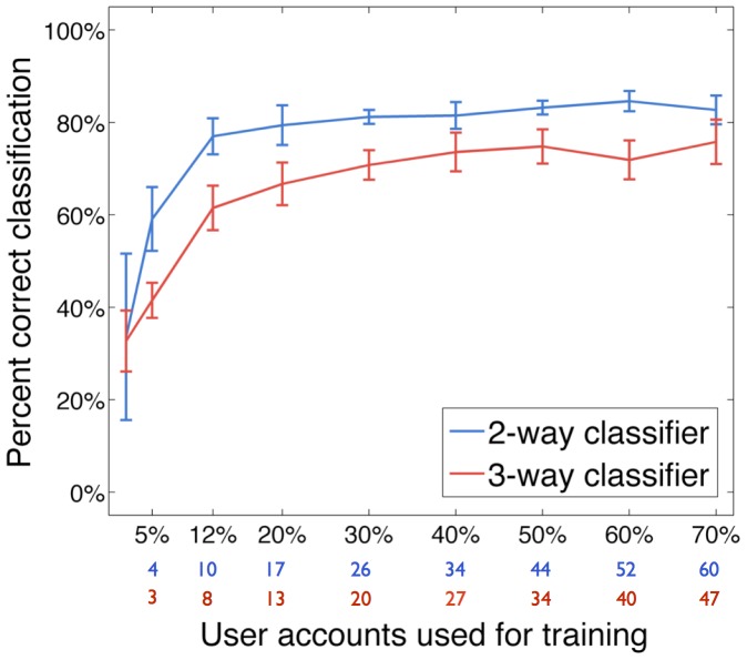
Human behaviour is highly individual by nature, yet statistical structures are emerging which seem to govern the actions of human beings collectively. Here we search for universal statistical laws dictating the timing of human actions in communication decisions. We focus on the distribution of the time interval between messages in human broadcast communication, as documented in Twitter, and study a collection of over 160,000 tweets for three user categories: personal (controlled by one person), managed (typically PR agency controlled) and bot-controlled (automated system). To test our hypothesis, we investigate whether it is possible to differentiate between user types based on tweet timing behaviour, independently of the content in messages. For this purpose, we developed a system to process a large amount of tweets for reality mining and implemented two simple probabilistic inference algorithms: 1. a naive Bayes classifier, which distinguishes between two and three account categories with classification performance of 84.6% and 75.8%, respectively and 2. a prediction algorithm to estimate the time of a user's next tweet with an R(2) ≈ 0.7. Our results show that we can reliably distinguish between the three user categories as well as predict the distribution of a user's inter-message time with reasonable accuracy. More importantly, we identify a characteristic power-law decrease in the tail of inter-message time distribution by human users which is different from that obtained for managed and automated accounts. This result is evidence of a universal law that permeates the timing of human decisions in broadcast communication and extends the findings of several previous studies of peer-to-peer communication.

Figure 1. Plots illustrating the methods used for the computation and evaluation of the predictive algorithms.

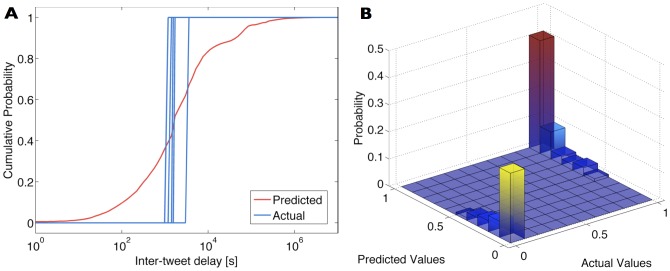
(a) The CDF computed for the personal accounts class using accounts is shown in red, while the step functions computed for 5 tweets of the left-out account are shown in blue. The CDF corresponds to the probability that a tweet will be posted seconds after the previous tweet (predicted probability), while the step functions correspond to the observed probability for the occurrence of tweets (observed or actual probability). A perfect prediction for a specific tweet would mean that the CDF coincides exactly with the step function for that tweet. (b) In this histogram, the axis on the left of the plane corresponds to the value of the CDF obtained for the inter-tweet delay (predicted value), while the axis on the right corresponds to the value of the step function obtained for the same delay (actual value, which is either 0 or 1). A perfect predictive model would have all data points grouped in bins and , indicating that the CDF models the step functions exactly and thus all predicted and actual values coincide. The fact that these two bins have much higher probabilities than all others in the histogram illustrates the model's accuracy.

Figure 2. Power spectral density estimation of tweeting activity for each class.

Log-log plots showing power spectral density (power per frequency in units of dB/Hz) vs. frequency (Hz) for each account class. This scale-free relationship suggests that there are no relevant dominant frequencies in tweeting activity.

Figure 3. Scatter plots of inter-tweet delay standard deviation vs. mean.

Scatter plots showing, for each individual, the inter-tweet delay standard deviation vs. the inter-tweet delay mean (A: 86 personal accounts, B: 91 managed accounts, C: 67 bot accounts). Linear fits (the black line denotes the unit slope) show that variability of inter-tweet delay is closely proportional to mean inter-tweet delay, i.e. inter-tweet delays exhibit signal-dependent noise characteristics.

Figure 4. Distributions for the inter-tweet delay and fitted power-laws.

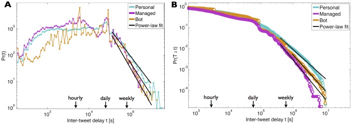
(a) Probability density function (PDF) for the inter-tweet delay of each class. The distributions were created using 100 logarithmically spaced bins between decades and . The power-laws fitted to the tails of the distributions have an exponent for personal accounts, for managed accounts, and for bot-controlled accounts. (b) The complementary cumulative distribution function (CCDF) for the inter-tweet delay in each class is shown along with the power-law distribution fitted to the tail. The full statistics of the power-law fits are presented in Table 2.

Figure 5. Polar plots of mean tweet time of the day and variability.

Polar plots showing, for each individual of each class (A: 86 personal accounts, B: 91 managed accounts, C: 67 bot accounts) on the polar axis the mean tweet time hour of the day (in local time zone) and on the radial axis the circular dispersion of the von Mises distribution (equivalent to the standard deviation). Note that the three subfigures have different dispersion ranges.

Figure 6. Probability density functions for tweet times.

The horizontal axis corresponds to the hours of the day, in hourly bins from 0 (midnight) to 23 h (11pm). All timestamps are in the local time zone of each user.

Figure 7. Number of tweets on each day of the week for each account class.

Rows correspond to 65 individual accounts and columns correspond to the days of the week. The mean tweet count for each tile is represented by the colour scale. The 65 most active accounts from each class are shown, and users are sorted by increasing total number of tweets collected, thus accounts have the same order as in Figure 8.

Figure 8. Number of tweets at each hour for each account class.

Rows correspond to 65 individual accounts and columns correspond to the hours of the day. The mean tweet count for each tile is represented by the colour scale. The 65 most active accounts from each class are shown, and users are sorted by increasing total number of tweets collected, thus accounts have the same order as in Figure 7.

Figure 9. Classification correctness obtained with varying training dataset size.

We evaluated the robustness of our classification algorithms by testing with different sizes for the training and test datasets. The horizontal axis shows the percentage of user accounts used for training, as well as the number of accounts used for training in the 2-Classifier (in blue) and in the 3-Classifier (in red). The remaining accounts were used for testing. Both algorithms perform well above a randomised model in all experiments, even when the training dataset comprised only 30% of the samples (81.2% vs. 52.2% for the 2-Classifier, and 70.8% vs. 32.3% for the 3-Classifier). In these experiments, we used the joint distribution of inter-tweet delay and tweet time as independent variables, and used a total of 86 accounts from each class in the 2-Classifier and 67 accounts from each class in the 3-Classifier. Each experiment was repeated 10 times, and at each time the samples were randomly shuffled among each class.

References

-
- Paul MJ, Dredze M (2011) You are what you tweet: Analyzing Twitter for public health. In: Proceedings of the Fifth International AAAI Conference on Weblogs and Social Media (ICWSM). pp. 265–272.
- Bollen J, Pepe A, Mao H (2009). Modeling public mood and emotion: Twitter sentiment and socio-economic phenomena.
Publication types
MeSH terms
LinkOut - more resources
Full Text Sources
Other Literature Sources
Research Materials