Specific evidence of low-dimensional continuous attractor dynamics in grid cells

Abstract

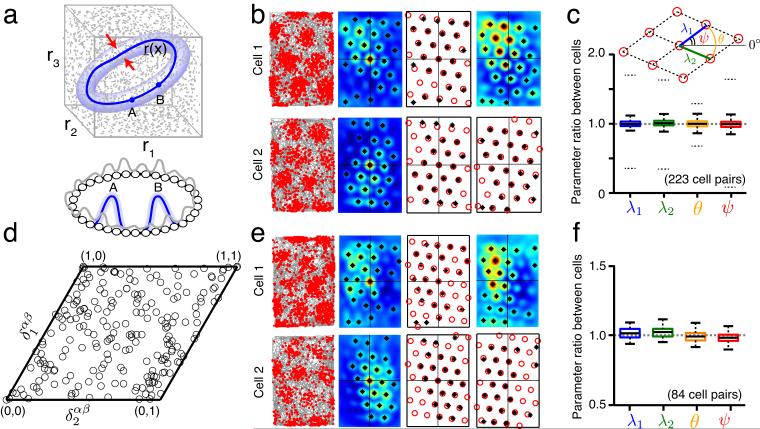
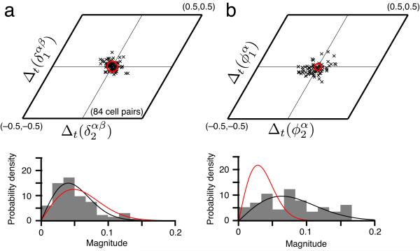
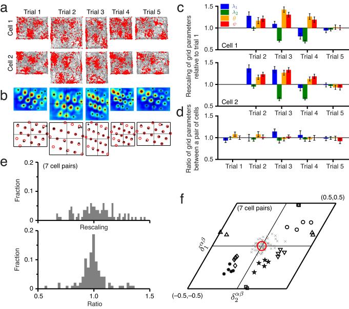
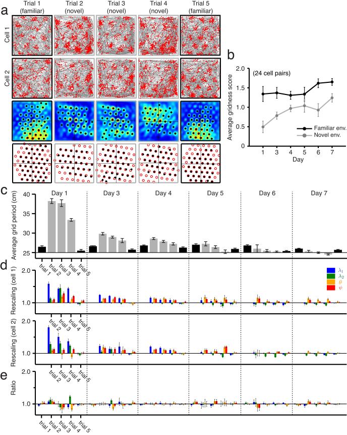
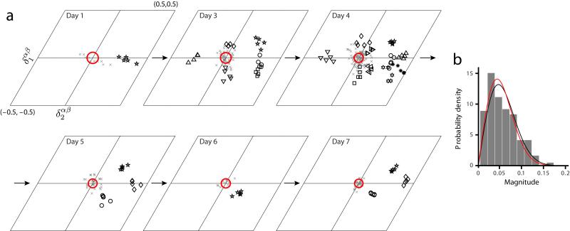
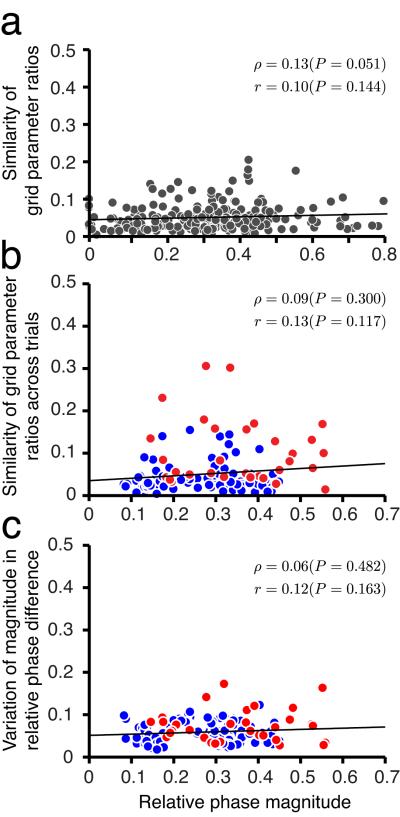
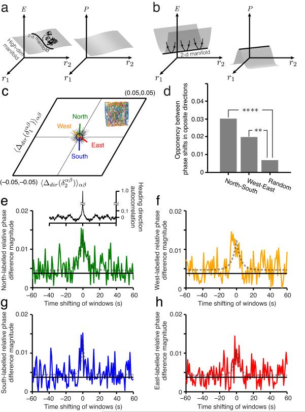
We examined simultaneously recorded spikes from multiple rat grid cells, to explain mechanisms underlying their activity. Among grid cells with similar spatial periods, the population activity was confined to lie close to a two-dimensional (2D) manifold: grid cells differed only along two dimensions of their responses and otherwise were nearly identical. Relationships between cell pairs were conserved despite extensive deformations of single-neuron responses. Results from novel environments suggest such structure is not inherited from hippocampal or external sensory inputs. Across conditions, cell-cell relationships are better conserved than responses of single cells. Finally, the system is continually subject to perturbations that, were the 2D manifold not attractive, would drive the system to inhabit a different region of state space than observed. These findings have strong implications for theories of grid-cell activity and substantiate the general hypothesis that the brain computes using low-dimensional continuous attractors.

Figure 1

Spatial grid parameters other than phase are identical across cells recorded on the same or nearby tetrodes; cell-cell relationships are stable over time. (a) Top (state space): The state of N independent neurons, each described by a firing rate r_i in [0, r_max] may lie anywhere in an N -dimensional cube of side length r_max□ (shown for N = 3 neurons). Appropriate coupling between the neurons can shrink the allowed states to a low-dimensional attractor (dark blue). All other states are transient, rapidly decaying back to the attractor, and are thus rarely seen. States very close to the attractor (light blue), through transient, may be observed if perturbations frequently drive the system into those states. Bottom: An example network of N neurons (small circles) with 1-d continuous attractor dynamics. Local excitatory and global inhibitory connections (not shown) between all neurons stabilize population states that are local activity bumps (e.g. blue bump A or B; gray: transient/unstable activity profiles). An activity bump is a single point on the continuous attractor (top) of all possible translations of the bump. If points on the attractor are identified with values of some circular variable, then all neural tuning curves for that variable will be identical, except for a phase shift (translation). (b) Column one: Recorded spikes (red dots) of two simultaneously recorded cells as a function of space (rat trajectory: gray lines). Column two: Autocorrelograms of the smoothed spatial response (peaks identified by black asterisks). Column three: A template lattice (red circles) is fit to all the peaks of the autocorrelogram. Parameters of the template (see c, inset) include the two primary axis lengths (λ₁,λ₂) and two angles (θ,ψ). Column four: Crosscorrelogram between the two cells (top), and the corresponding template fit (bottom). (c) Box plot of the ratio of each lattice parameter across 223 cell pairs (e.g., θ” (cell ” i)/θ” (cell ” j)” where ” i > j ) (median ratio: center line in box; interquartile ranges: box; lowest and highest values within 1.5 × of interquartile range: outer horizontal lines; 95% confidence interval based on 223 randomly chosen pairs not recorded simultaneously: dotted outer horizontal lines). (d) The distribution of relative phases (black circles) between all cell pairs, plotted within a canonical unit cell of the grid lattice. (e) Discharge maps (as in b) of the same cell pair, recorded again after an interval of > 60 minutes. (f) Box plot of parameter ratios (as in c) from this later trial, for the subset of cell pairs from c that were also recorded in this trial (N = 84 cell pairs).

Figure 2

Across time in familiar environments, the relative phases between cells are more stable than the phases of single cells. (a) Top: The difference across time (trials separated by > 60 mins) in the relative phase between cell pairs is clustered near zero (black x’s, see Online Methods). Red circle: uncertainty in estimating relative phase differences (see Online Methods for error analysis). Bottom: Normalized histogram of the magnitudes of these relative phase differences (gray), with the null distribution (red), in which phase differences are not significantly different from zero and drawn independently from a Gaussian with standard deviation equal to the uncertainty in phase estimation. The null distribution of magnitudes is Rayleigh. Black: best-fit Rayleigh distribution to the data. (b) Difference across time (i.e., trials) of the phase of single cells (top), and the normalized histogram of magnitudes (bottom). Black, red defined similarly as in a. The data in a are not significantly different from the null hypothesis, while those in b are (a: P = 0.58 » 0.05, b: P « 10–4 under the F-test for whether the data and the null distribution come from a distribution of the same variance). Finally, P < 0.001 under the F-test for whether the data in a, b (bottom) come from a distribution of the same variance.

Figure 3

Grid parameter ratios and relative phases are stable even when grid parameters are rescaled as the environment is resized. (a) Firing fields of two simultaneously recorded cells in a familiar environment (trials 1, 5) and resized versions of the familiar environments (trials 2, 3, and 4). (b) Spatial crosscorrelograms for the cell pair (top) and the best-fit template lattices (bottom). Asterisks denote local peaks in the crosscorrelogram. (c) Each grid parameter for cell 1 (top) or cell 2 (bottom) normalized by the value from trial 1. The parameters are substantially rescaled across trials 2–4.Error bars indicate ± 1 s.d. (Online Methods). (d) The ratio, between cells 1 and 2, of each grid parameter, for each trial. The ratios are statistically very close to one, despite the significant rescaling in each cell, seen in c. Error bars indicate 1 ± s.d. (Online Methods). (e) Top: Histogram of all grid parameters for the 11 cells in the resizing experiments from trials 2,3,4 normalized to the corresponding value from trial 1. Bottom: Histogram of the ratios of all grid parameter values between cells 1 and 2 for all 7 cell pairs from trials 1–4. This distribution is strongly peaked at 1 and different from the distribution at top. The Kolmogorov-Smirnov test for whether the two data samples come from the same distribution produces P < 0.001. The F-test for whether the two data samples come from a distribution of the same variance produces P < 0.001. (f) The relative phases for the 7 cell pairs span the unit cell (each black symbol represents a different cell pair; each marker for a given symbol represents a different trial). Gray x’s: relative phase differences, computed across all cell pairs and trials. Red circle: uncertainty in the relative phase difference magnitude (Online Methods). The relative phase differences are not significantly different from zero (P ≈ 0.6 » 0.05 for the same null hypothesis as in Fig. 2).

Figure 4

Grids become less stable and expand in novel enclosures, but grid parameter ratios remain stable. (a) Firing fields of pairs of simultaneously recorded cells in a familiar environment (black squares) and novel ones (gray squares) across five consecutive trials on one day, and the corresponding crosscorrelograms and best-fit template lattices. Note that on different days, the recordings involve different cells from the same tetrodes in the same area in the animal (Supplementary Fig. 5 for all cell pairs). (b) Development of average modified gridness in novel environments (gray) across seven days. The grid score gradually approaches that measured in familiar environments (black) (24 cell pairs, from ref. ; means ± s.e.m.). (c) Change, across trials and days in the novel environment (gray), of the average grid period. Average grid period is the mean of the first two grid parameters across all cells in a trial (means ± s.e.m. 24 cell pairs total: 1, 6, 10, 3, 1, and 3 on days 1, 3, 4, 5, 6, and 7, respectively; no cells in day 2 passed the gridness criterion). The grid period significantly rescales in a novel environment, compared to when measured in the familiar environment (black), then gradually relaxes to its original value over seven days. (d) Grid parameters of one typical cell pair from each day (all cell pairs shown in Supplementary Fig. 5), normalized by the corresponding parameter values from the first trial (familiar environment) of the day. Clusters of four narrow bars represent the four parameters, in the same ordering and color scheme as in Figs. 1 and 3. Error bars indicate ± 1 s.d. (Online Methods). (e) Grid parameter ratios for the two cells, across trials and days. Almost all these ratios are statistically indistinguishable from 1 (for all cell pairs, see Supplementary Figs. 5 and 6). Error bars indicate ± 1 s.d. (Online Methods).

Figure 5

Relative phase remains stable in novel enclosures. (a) The relative phases of the cell pairs (each distinct symbol represents a pair), across different trials and days (N = 24 cell pairs from ref. , across all 7 days). Gray x’s: the relative phase difference for every trial and all pairs. Red circle: uncertainty in the magnitude of relative phase differences (Online Methods). (b) The relative phase differences are not significantly different from zero for the same null hypothesis as in Fig. 2 (P = 0.38 » 0.05 under the F-test for whether the data and the null distribution come from a distribution of the same variance).

Figure 6

Stability of cell-cell relationships is independent of distance in spatial phase. (a) Parameters between cell pairs (223 cell pairs from Fig. 1c,d) in the same network are very similar (as reported in Fig. 1), and moreover, the degree of similarity does not vary with the difference in spatial phase (i.e. magnitude of relative phase) between cells (Parameter similarity is defined as the square-root of the squared deviation of parameter ratios from 1, averaged over all parameters per pair). Each dot represents one trial from one cell pair. Black: linear regression; p : Spearman’s rank correlation; r : Pearson’s product-moment correlation. (b) The stability of parameter ratios between cell pairs across rescaling trials (red dots, 7 pairs from Fig. 3f) and novel enclosure trials (blue dots, 24 pairs from Figs. 4 and 5) is independent of the pair’s relative phase. (c) The stability of relative phase (mean of magnitude of relative phase differences) across rescaling and novel enclosure trials is independent of relative phase between cells in a pair (same dataset and color-coding as in b).

Figure 7

Evidence of external perturbation and attractor dynamics in grid cell activity (a-b) Schematic energy landscape (left) and occupation probability (right) plots of a dynamical system. The independent variables on the plots depicting energy (left) and probability density (right) as heights are the firing rates of the neurons in the network. If the energy landscape has a flat plateau (a, left) of dimension D > 2, in which the 2-d manifold is embedded (depicted as a line), the system will likely be found off the 2-d manifold because there is no specific restoring drive back to it (a, right). When there is a 2-d valley in energy (b, left), the system state will be localized to the 2-d manifold (b, right) even in the presence of noise. (c) Inset: animal trajectory from one trial color-coded (green, blue, red, yellow) by the instantaneous movement direction (North, South, East, West quadrants, respectively). Main plot, green vector: the difference in relative phase between cell pairs, computed as the relative phase obtained from spikes obtained only during Northward trajectory fragments minus the relative phase obtained from all spikes in the trajectory, averaged across all cell pairs (223 pairs). Gray vectors: Samples from the null hypothesis of randomly segmenting the full trajectory into four sets of fragments of the same average lengths as the directional fragments, without directional specificity. Black circle: one standard deviation of the null hypothesis distribution (Online Methods). p -values for the directional shifts in relative phase under null hypothesis: North (P = 0.0004), West (P = 0.0444), South (P = 0.0003), East (P = 0.0201). (d) Opposing shifts in relative phase from opposing trajectory directions: North-South (****P < 10⁻⁴), West-East (**P < 0.0014 ) (Online Methods). (e-h) Green: Directional shifts induced in relative phase decay as the spike selection windows spanning Northward trajectory fragments are shifted in time, 1 second at a time, away from the centers of those directional segments, to include spikes emitted just before or after Northward movements. Black solid line: Radius of black circle from c. Gray dotted curve: Best-fit Laplace distribution with zero mean. Inset: Autocorrelation of movement direction in trajectories.

References

1. Hopfield J. Neural networks and physical systems with emergent collective computational abilities. Proceedings of the National Academy of Sciences. 1982;79:2554. - PMC - PubMed
1. Ben-Yishai R, Bar-Or R, Sompolinsky H. Theory of orientation tuning in visual cortex. Proceedings of the National Academy of Sciences. 1995;92:3844. - PMC - PubMed
1. Seung HS. How the brain keeps the eyes still. Proceedings of the National Academy of Sciences. 1996;93:13339–13344. - PMC - PubMed
1. Zhang K. Representation of spatial orientation by the intrinsic dynamics of the head-direction cell ensemble: a theory. J. Neurosci. 1996;16:2112–2126. - PMC - PubMed
1. Seung HS, Lee D. The manifold ways of perception. Science. 2000;290:2268–2269. - PubMed
Publication types