Inferring nonlinear neuronal computation based on physiologically plausible inputs

Abstract

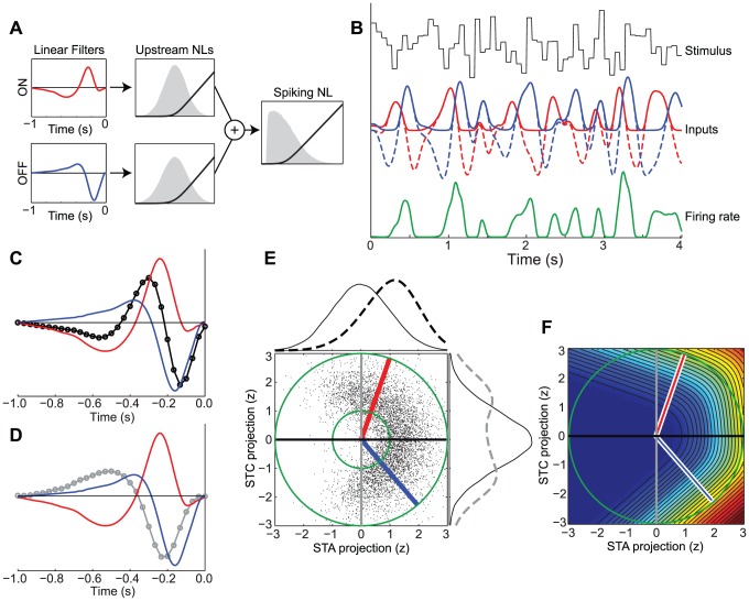
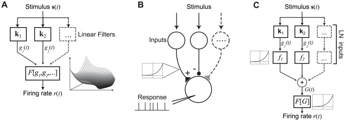
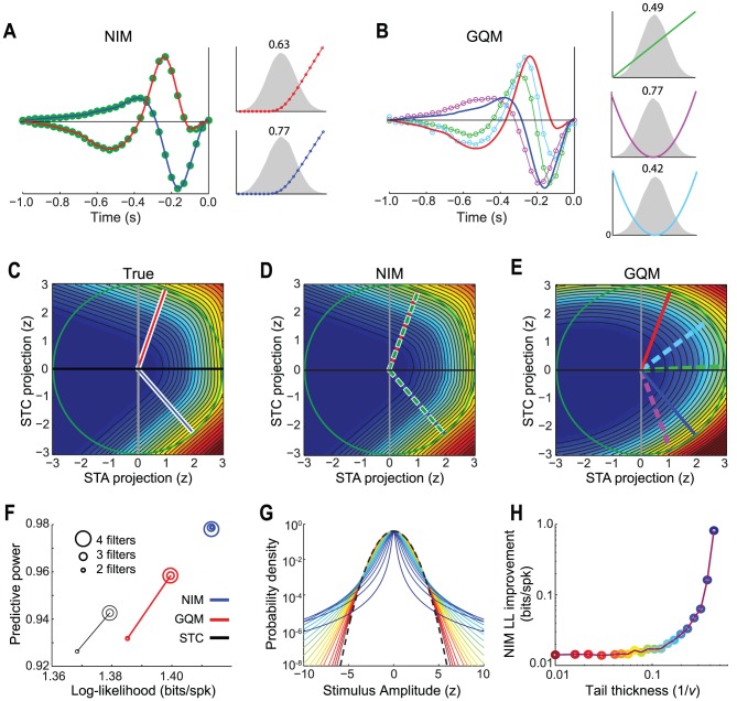
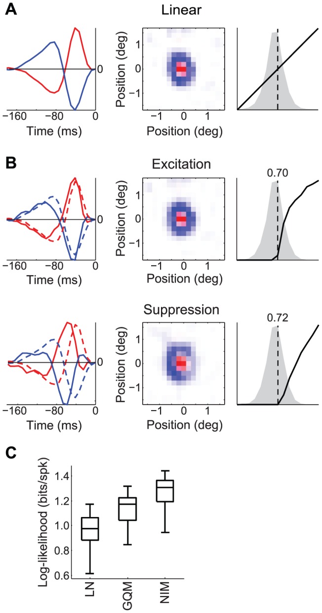
The computation represented by a sensory neuron's response to stimuli is constructed from an array of physiological processes both belonging to that neuron and inherited from its inputs. Although many of these physiological processes are known to be nonlinear, linear approximations are commonly used to describe the stimulus selectivity of sensory neurons (i.e., linear receptive fields). Here we present an approach for modeling sensory processing, termed the Nonlinear Input Model (NIM), which is based on the hypothesis that the dominant nonlinearities imposed by physiological mechanisms arise from rectification of a neuron's inputs. Incorporating such 'upstream nonlinearities' within the standard linear-nonlinear (LN) cascade modeling structure implicitly allows for the identification of multiple stimulus features driving a neuron's response, which become directly interpretable as either excitatory or inhibitory. Because its form is analogous to an integrate-and-fire neuron receiving excitatory and inhibitory inputs, model fitting can be guided by prior knowledge about the inputs to a given neuron, and elements of the resulting model can often result in specific physiological predictions. Furthermore, by providing an explicit probabilistic model with a relatively simple nonlinear structure, its parameters can be efficiently optimized and appropriately regularized. Parameter estimation is robust and efficient even with large numbers of model components and in the context of high-dimensional stimuli with complex statistical structure (e.g. natural stimuli). We describe detailed methods for estimating the model parameters, and illustrate the advantages of the NIM using a range of example sensory neurons in the visual and auditory systems. We thus present a modeling framework that can capture a broad range of nonlinear response functions while providing physiologically interpretable descriptions of neural computation.

Figure 1. ON-OFF RGC simulation.

A) Schematic showing the ON (top, red) and OFF (bottom, blue) inputs to the simulated ON-OFF RGC. The temporal filters (left) process the stimulus, and the upstream nonlinearities (black, middle) are then applied to the filter outputs. The sum of the two inputs is then passed through the spiking nonlinearity (black, right). The distributions of the stimulus filtered by the ON and OFF pathways, as well as the distribution of their summed input to the simulated neuron are shown as gray shaded regions. B) A simulation showing how the response to a 15 Hz (Gaussian) white noise stimulus is constructed. The stimulus (black) is filtered by the ON and OFF temporal kernels (dashed red and blue), and then transformed by the upstream nonlinearities (solid red and blue). The resulting instantaneous firing rate (green) is given by the sum of these inputs passed through the spiking nonlinearity. C) The STA (black) resembles the average of separate ON (red) and OFF (blue) filters of the generative model. D) Similar to panel C, the first STC filter (gray) resembles a mixture of the ON and OFF filters. E) Stimuli eliciting spikes (black dots) are projected onto the two-dimensional subspace spanned by the STA and first STC filter, shown in units of z-score. The distributions of stimuli corresponding to spikes (dashed lines on top and left) are compared to the marginal stimulus distributions (solid), demonstrating a systematic bias along the STA (horizontal) axis, and an increased variance along the STC (vertical) axis. The true ON and OFF filters (red and blue) are also contained in the STA/STC subspace, as indicated by the red and blue lines lying on the unit circle (green). The inner green circle has a radius of one standard deviation. F) The neuron's firing rate as a function of the stimulus projected into the 2-D STA/STC subspace (shaded color depicts firing rate: increasing from blue to red).

Figure 2. Schematic of LN and NIM structures.

A) Schematic diagram of an LN model, with multiple filters (k₁, k₂, …) that define the linear stimulus subspace. The outputs of these linear filters (g ₁, g ₂, …) are then transformed into a firing rate prediction r(t) by the static nonlinear function F[g ₁,g ₂,…], depicted at right for a two-dimensional subspace. Note that while the general LN model thus allows for a nonlinear dependence on multiple stimulus dimensions, estimation of the function F[.] is typically only feasible for low (one- or two-) dimensional subspaces. B) Schematic illustration of a generic neuron that receives input from a set of ‘upstream’ neurons that are themselves driven by the stimulus s. Each of the upstream neurons provides input to the model neuron that is generally rectified due to spike generation (inset at left), and thus is either excitatory or inhibitory. The model neuron then integrates its inputs and produces a spiking output. C) Block diagram illustrating the structure of the NIM, based on (B). The set of inputs are represented as (one-dimensional) LN models, with a corresponding stimulus filter k_i, and “upstream nonlinearity” f_i(.). These inputs are then linearly combined, with weights w _i, and fed into the spiking nonlinearity F[.], resulting in the predicted firing rate r(t). The NIM thus has a ‘second-order LN’ structure (or LNLN), with the neuron's own nonlinear processing shaped by the LN nature of its inputs.

Figure 3. Comparison of NIM and quadratic model.

A) The filters fit by the NIM (green dots) are able to capture the true underlying ON and OFF filters (red and blue), as well as the shape of the upstream nonlinearities (right), which are shown relative to the corresponding distributions of the filtered stimulus (gray shaded). The ranges of the y-axes for different subunits are indicated by the numbers above, for comparison of their relative magnitudes. These ‘subunit weights’ are scaled so that their squared magnitude is one. B) The filters fit by the GQM, consisting of two (excitatory) squared filters (magenta and light blue) and a linear filter (green trace), are different than the true filters (red and blue), but are in the same subspace, as demonstrated in (E). C) The simulated neuron's response function (shaded color depicts firing rate) and true filters (red and blue) projected into the STC subspace (identical to Fig. 1F). D) Response function predicted by the NIM. The filters identified by the NIM (dashed green) overlay onto the true filters. E) Same as (D) for the GQM, with colored lines corresponding to the filters in (B). F) Model performance is plotted for the STC, GQM, and NIM fit with different numbers of filters (indicated by different circle sizes). Log-likelihood (relative to the null model) is shown on the x-axis, and the ‘predictive power’ is shown on the y-axis; both were evaluated on a simulated cross-validation data set. The NIM (blue) outperforms the GQM (red), both of which outperform a nonlinear model based on the STC filters (black, see Methods). The STC model and GQM achieve maximal performance with 3 filters, since this is sufficient for capturing the best-fit quadratic function in the relevant 2-D stimulus subspace, while the NIM achieves optimal performance with two filters, as expected. G) To determine how model performance depends on the stimulus distribution we simulated the same neuron's response to white noise luminance stimuli with Student's t-distributions, ranging from Gaussian (i.e., ν = ∞, dashed black) to “heavy tailed” (decreasing ν from red to blue). H) The log-likelihood improvement of the NIM over the GQM increases as a function of the tail thickness (parameterized by 1/ν) of the stimulus distribution (which also determines the tail thickness of the filtered stimulus distributions). The GQM is able to provide a very close approximation for large values of v (i.e., a more normally-distributed stimulus), but has lower performance compared to the NIM for more heavy-tailed stimuli.

Figure 4. Spatiotemporal tuning of excitatory and suppressive inputs to an LGN neuron.

A) The linear receptive field can be represented as the sum of two space-time separable components, corresponding to the receptive field center (red) and surround (blue). B) The NIM with excitatory (top) and suppressive (i.e., putative inhibitory, bottom) inputs. The excitatory and suppressive components (solid) both have slower, and less biphasic, temporal responses (left) compared with the linear model (dashed). The suppressive input is also delayed relative to the excitatory input. Both excitatory and suppressive inputs have roughly the same spatial profiles (middle), and both provide rectified input through the corresponding upstream nonlinearities (right). C) The NIM has significantly better performance, as measured by cross-validated log-likelihood, compared to the linear model (p = 0.002; n = 10 cross-validation sets; Wilcoxon signed rank test) and the GQM (p = 0.002).

Figure 5. Spectrotemporal tuning of excitation and suppression in the songbird auditory midbrain.

A) The linear spectrotemporal receptive field (STRF; left) contains two subfields of opposite sign. B) The excitatory (top) and suppressive (bottom) spectrotemporal filters identified by the NIM are similar to the positive and negative subfields of the linear STRF respectively. However, these inputs are both rectified by the upstream nonlinearities (right), resulting in different stimulus processing (see Fig. S4). C) Comparison of log-likelihoods of the LN model, GQM, and NIM. Red lines show the performance across models for each cross-validation set. Note that the duration of the recording, and the neuron's relatively low firing rate, limit the statistical power of model comparisons.

Figure 6. Modeling stimulus selectivity arising from many inputs.

A) Simulated V1 neurons are presented with one-dimensional spatiotemporal white noise stimuli (left). Their stimulus processing is constructed from a set of spatiotemporal filters (example shown at right), depicted with one spatial dimension (x-axis) and time lag (y-axis). B) The first simulated neuron is constructed from six spatially overlapping direction-selective filters (top), similar to those observed experimentally for V1 neurons. Below, the corresponding filtered stimulus distributions are shown along with the respective upstream nonlinearities (blue). C) The NIM identifies the correct spatiotemporal filters (top), as well as the form of the upstream nonlinearities (middle). The projections of the NIM filters onto the true filters (bottom) illustrate that the NIM identifies the true filters. D) The STA for the simulated neuron (left), along with the three significant STC filters (right) are largely contained in the subspace spanned by the true filters, but reflect non-trivial linear combinations of these filters (bottom). E) The GQM is composed of a linear input (left) and three excitatory squared inputs (right). While the GQM filters are more similar to the true filters, they also represent non-trivial linear combinations of them (bottom). F) The second simulated neuron consists of four similar, but spatially shifted, inputs that are squared. G) The NIM represents each true (squared) input by an opposing pair of rectified inputs. H) The STA (left) does not show any structure because the neuron's response is, by construction, symmetric in the stimulus. The four significant STC filters (right) represent distributed linear combinations of the four underlying filters. I) The GQM recovers the correct stimulus filters, given appropriate sparseness regularization.

Figure 7. Models of multi-input stimulus processing in a V1 neuron.

A) Standard spike-triggered characterization for this neuron reveals a ‘complicated simple-cell’ response , with a clear direction-selective STA (left), two excitatory STC filters (middle), and six suppressive STC filters (right). B) The GQM identifies a set of filters (one linear, two squared excitatory, and six squared suppressive) that are roughly similar to the STA/STC filters, but with smoother and sparser spatiotemporal structure (due to regularization). C) The NIM filters (top) and upstream nonlinearities (bottom) reveal a similar description of the stimulus processing, although with greater consistency among the (six) excitatory and (six) suppressive stimulus filters. D) Comparison of the cross-validated log-likelihood of the LN model (one linear filter), the ‘STC model’ given by fitting a GLM to the outputs of the STA/STC filters (see Methods), the GQM, and the NIM. Given the neuron's simple-cell-like response (i.e., large weight of the STA), a large fraction of the response can be captured with the linear filter alone (the LN model). Nevertheless, all three multi-filter models provide substantial improvements compared to the LN model. E) In order to compare the performance of the nonlinear (multi-filter) models directly, their improvement relative to the LN model is depicted. This shows that the GQM significantly outperforms the ‘STC’ model (p = 0.002; n = 10; Wilcoxon signed rank test), and that the NIM similarly outperforms the GQM (p = 0.002).

Figure 8. Models of a V1 neuron in the context of natural stimuli.

A) The natural movie stimulus used here has two spatial and one temporal dimension. B) The neuron's response is characterized in terms of three-dimensional spatiotemporal filters. An example spatiotemporal filter is comprised of a spatial filter at each time step (at 20 ms resolution). To simplify the depiction of each filter, we take advantage of their stereotyped structure, and plot the spatial distribution at the best time slice (BTS, left), as well as the space-time projection (STP, right) along an axis orthogonal to the preferred orientation (red line; see Methods). C) The GQM for this neuron consists of one linear (top) and two excitatory squared filters (bottom). The BTS and STP for each filter are shown at left, and the distributions of the filtered stimulus, and associated nonlinearities, are shown at right. Note that the two squared filters roughly form a ‘quadrature pair’ of direction-selective Gabor filters. There is also a linear filter (top), which has less clear spatial structure, and is not direction-selective. D) The NIM consists of four excitatory filters (left) that are qualitatively similar to the quadrature pair of GQM filters. However, by identifying four inputs with inferred upstream nonlinearities (right), the NIM has greater flexibility in describing the neuron's computation. E) Comparison of model performance for the LN and STC-based models, as well as the GQM and NIM, showing that the NIM substantially outperformed other models for this neuron.

References

1. Riesenhuber M, Poggio T (1999) Hierarchical models of object recognition in cortex. Nat Neurosci 2: 1019–1025. - PubMed
1. Brincat SL, Connor CE (2004) Underlying principles of visual shape selectivity in posterior inferotemporal cortex. Nat Neurosci 7: 880–886. - PubMed
1. Mineault PJ, Khawaja FA, Butts DA, Pack CC (2012) Hierarchical processing of complex motion along the primate dorsal visual pathway. Proc Natl Acad Sci U S A 109: E972–E980. - PMC - PubMed
1. DiCarlo JJ, Cox DD (2007) Untangling invariant object recognition. Trends Cogn Sci 11: 333–341. - PubMed
1. Rust NC, Stocker AA (2010) Ambiguity and invariance: two fundamental challenges for visual processing. Curr Opin Neurobiol 20: 382–388. - PubMed
Publication types
MeSH terms
LinkOut - more resources