High-speed panoramic light-sheet microscopy reveals global endodermal cell dynamics

Abstract

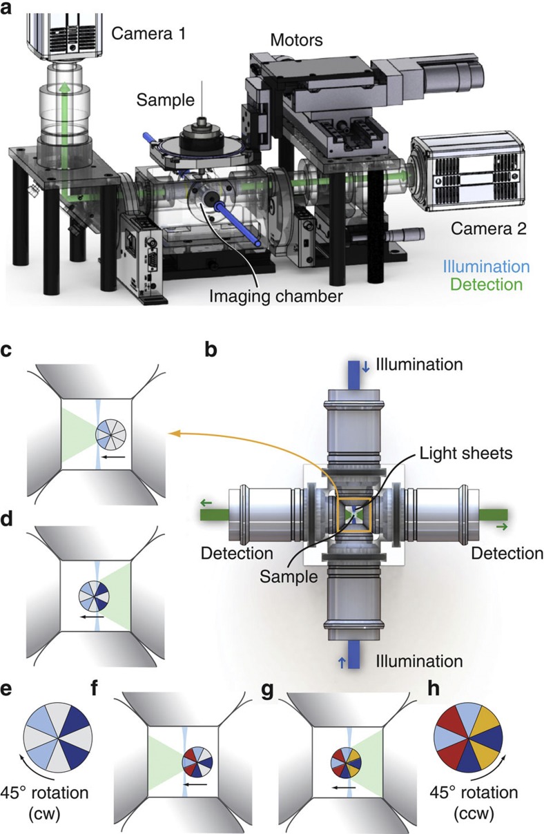
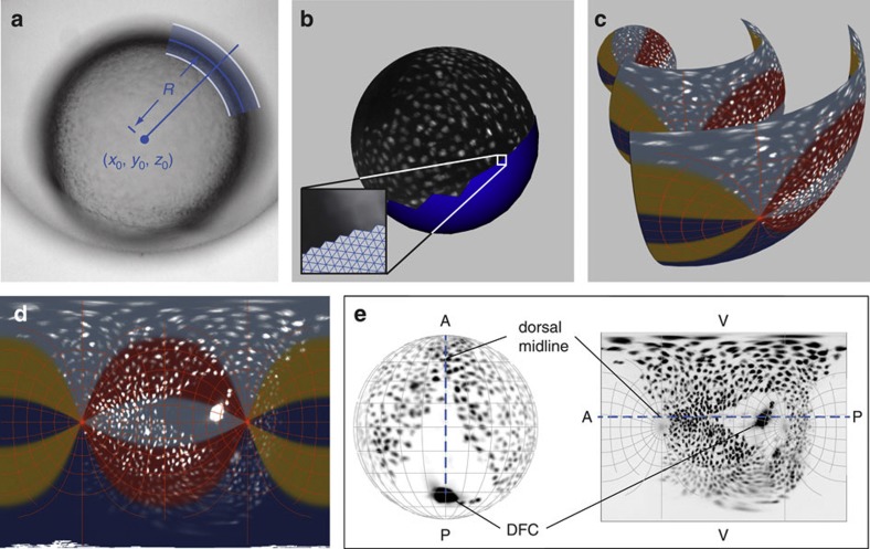
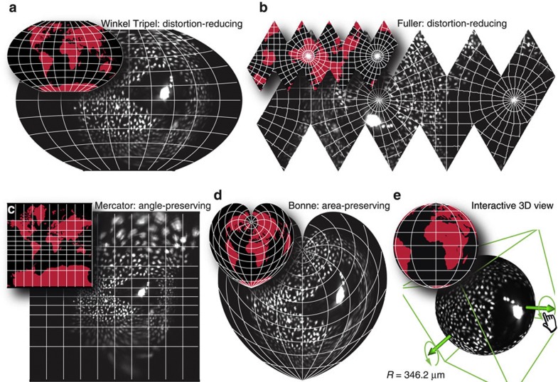
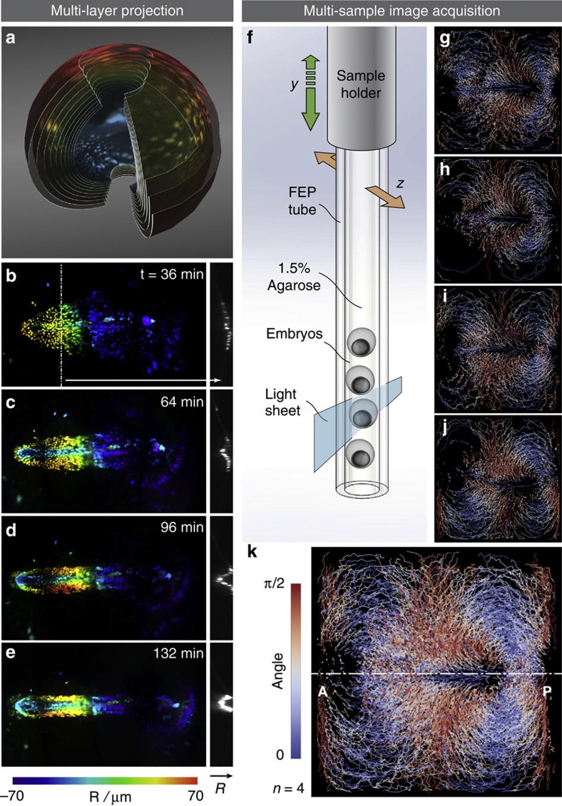
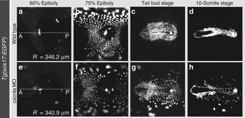
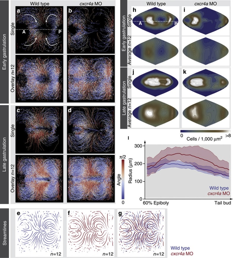
The ever-increasing speed and resolution of modern microscopes make the storage and post-processing of images challenging and prevent thorough statistical analyses in developmental biology. Here, instead of deploying massive storage and computing power, we exploit the spherical geometry of zebrafish embryos by computing a radial maximum intensity projection in real time with a 240-fold reduction in data rate. In our four-lens selective plane illumination microscope (SPIM) setup the development of multiple embryos is recorded in parallel and a map of all labelled cells is obtained for each embryo in <10 s. In these panoramic projections, cell segmentation and flow analysis reveal characteristic migration patterns and global tissue remodelling in the early endoderm. Merging data from many samples uncover stereotypic patterns that are fundamental to endoderm development in every embryo. We demonstrate that processing and compressing raw image data in real time is not only efficient but indispensable for image-based systems biology.

Figure 1. Four-lens SPIM setup and image acquisition.

(a) Schematic of the central unit of the four-lens SPIM setup. The sample dips into the medium-filled imaging chamber from the top. It is held and moved by a fast rotational stage and three linear motors. Light-sheets illuminate the sample from two opposite sides (blue arrows) and two cameras record the fluorescent signal orthogonally to the light sheets (green arrows). The cameras are precisely aligned to image the same plane. (b) The central imaging chamber consists of four identical lenses for two-sided illumination and two-sided detection of the sample (view from the top). The illumination objectives alternately excite the shared focal plane of the two detection lenses. (c–h) Steps involved in image acquisition. (c) As the sample is moved through the light sheet (arrow), two sectors are well illuminated and detected by the left detection arm (light blue). (d) During the second half of the stack, the right detection arm acquires parts on the right (dark blue). (e) The sample is rotated by 45° and (f,g) complementary regions are imaged in a similar manner (red and yellow), covering the entire sample. (h) The sample is rotated back by 45° and these steps are repeated for time-lapse acquisition (see also Supplementary Movie 1).

Figure 2. Spherical projection and real-time processing.

(a) A sphere is fitted to a series of transmission images of a zebrafish embryo. The coordinates of the centre (x₀, y₀, z₀) and the radius (R) are determined. A shell of 140 μm thickness around the sphere surface (blue shaded region) will contribute to the projection. (b) The surface of the sphere is divided into vertices (inset). A ray is cast from the sphere centre to each vertex, and the maximum intensity along each ray within the shell is recorded. (c) The resulting spherical maximum intensity projection is then unwrapped to obtain a 2D map of the spherical data (Supplementary Movie 2). Different colours indicate the parts of the embryo that were recorded by the two cameras from two different angles (compare Fig. 1). (d) All endodermal cells spread around the entire embryo are visible in a single image (Supplementary Movie 3). (e) Spatial orientation of the embryo in 3D and on the final map projection. A, anterior; P, posterior; V, ventral; DFC, dorsal forerunner cells.

Figure 3. Map projections to visualize the entire endoderm.

Various map projections are available to quantify different parameters and visualize patterns of cell organization (Supplementary Movie 6). (a,b) Winkel Tripel and Fuller projections show little distortion and are best suited to visualize the speed of cell migration. (c) Angle-preserving Mercator projections were used to visualize cell flows and direction of cell movement. (d) The Bonne projection is area preserving and was therefore used to depict cell densities. (e) Cell dynamics on the spherical data were also visualized interactively in Fiji’s 3D viewer²⁸, where the embryo can be turned to look at specific regions of interest. Insets in the top left corner depict the respective world map projections in red.

Figure 4. Multi-layer projections and multi-sample acquisition.

A multi-layer projection is created to capture the radial movement of cells during late gastrulation. (a) Rendering of a radial multi-layer projection, cut open to show the different layers, which are colour coded for different radii. (b–e) Time-lapse multi-layer Mercator projections of a late gastrulation stage embryo. Colour code indicates the radial position of cells from the innermost (blue) across 20 layers to the outermost (red) layer (Supplementary Movie 8). For comparison, cross-sections along the dotted line are shown on the right. (f) Schematic representation of multi-sample data acquisition. Multiple embryos are mounted in agarose in one FEP tube. A motor controls the position along y and positions each embryo in the light sheet in front of the objective lenses. Projections are then recorded by moving the embryo through the light sheet along z. (g–j) Four embryos were imaged in parallel (Supplementary Movie 9) and the cell tracks computed. Colour code indicates the unsigned angle between each track and the dorsal midline (dashed line in k). (k) Overlay of the cell tracks from g–j.

Figure 5. Visualizing endoderm cell dynamics in wild-type and crxcr4a morphant embryos.

Time-lapse images of the entire developing endoderm in Mercator projections. Tg(sox17:EGFP) line was used to visualize the endoderm from 60% epiboly to 10-somite stage (a–d) in wild type and (e–h) in crxcr4a morphant (Supplementary Movies 7 and 12). The radius of the fitted sphere (R) is stated for the individual data sets.

Figure 6. Quantification of endoderm cell dynamics reveals conserved flow patterns.

For quantitative analysis, movies were split into early (60–75% epiboly) and late gastrulation (75% epiboly, tail bud). (a–d) Orientation of cell migration (a,c) for wild type and (b,d) for cxcr4a morphants calculated on the angle-preserving Mercator projection (Supplementary Movies 11 and 13). Cell tracks from single embryos are shown on the top, the overlay of cell tracks from 12 embryos below. The colour scale indicates the unsigned angle between the cell track and the dorsal midline, direction of cell movement is indicated by white arrows in a. (e,f) Streamlines obtained from the cell tracks of multiple wild-type and cxcr4a morphant embryos to depict the overall flow pattern of endoderm cells during gastrulation. (g) Overlay of streamlines of wild type (blue) and cxcr4a morphants (red, n=12 each). Maps from different embryos were registered with the position of DFCs at tailbud stage for the overlay. (h–k) Spatial distribution of cells as kernel-density estimate on the area-preserving Bonne projections (h,j) for wild type and (i,k) for cxcr4a morphants (Supplementary Movie 14). Cell densities from single embryos are shown on the top, the averaged density distribution from 12 embryos below. The colour scale indicates local cell density from 0 to >8 cells/1,000 μm². (l) The distance between DFCs and the approaching endoderm margin during the course of gastrulation, obtained by calculating the 0.1 quantile of the cellular distributions in wild type (n=12, blue) and cxcr4a morphant (n=12, red) (Supplementary Fig. S8). The line graph represents the mean distance and the shaded region the standard deviation. In all images the equator corresponds to the dorsal midline, anterior to the left.

References

1. Lecuit T. Tissue Remodeling and Epithelial Morphogenesis. Current Topics in Developmental Biology Academic Press (2009).
1. Huisken J. & Stainier D. Y. R. Selective plane illumination microscopy techniques in developmental biology. Development 136, 1963–1975 (2009). - PMC - PubMed
1. Weber M. & Huisken J. Light sheet microscopy for real-time developmental biology. Curr. Opin. Genet. Dev. 21, 566–572 (2011). - PubMed
1. Huisken J., Swoger J., Del Bene F., Wittbrodt J. & Stelzer E. H. K. Optical sectioning deep inside live embryos by selective plane illumination microscopy. Science 305, 1007–1009 (2004). - PubMed
1. Swoger J., Verveer P. J., Greger K., Huisken J. & Stelzer E. H. K. Multi-view image fusion improves resolution in three-dimensional microscopy. Opt. Express 15, 8029–8042 (2007). - PubMed
Publication types