MACOP modular architecture with control primitives

Abstract

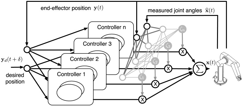
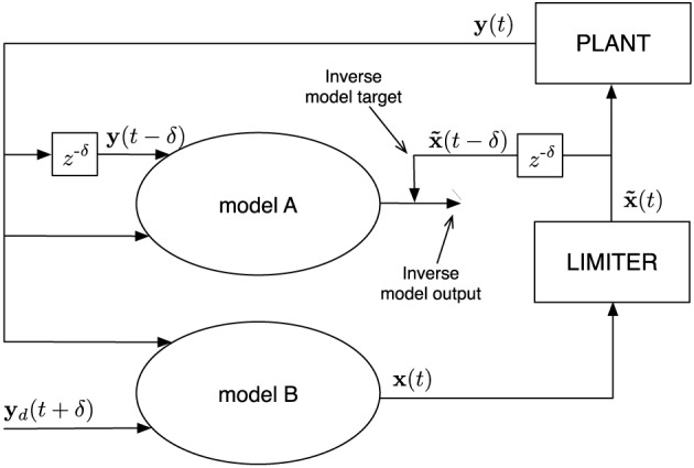
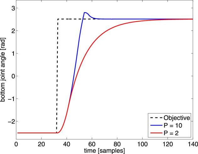
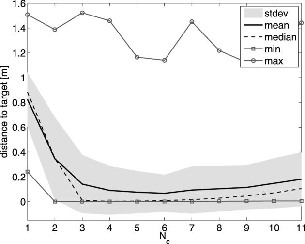
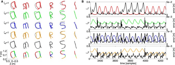
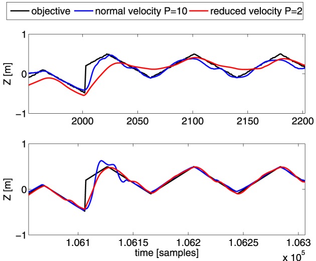
Walking, catching a ball and reaching are all tasks in which humans and animals exhibit advanced motor skills. Findings in biological research concerning motor control suggest a modular control hierarchy which combines movement/motor primitives into complex and natural movements. Engineers inspire their research on these findings in the quest for adaptive and skillful control for robots. In this work we propose a modular architecture with control primitives (MACOP) which uses a set of controllers, where each controller becomes specialized in a subregion of its joint and task-space. Instead of having a single controller being used in this subregion [such as MOSAIC (modular selection and identification for control) on which MACOP is inspired], MACOP relates more to the idea of continuously mixing a limited set of primitive controllers. By enforcing a set of desired properties on the mixing mechanism, a mixture of primitives emerges unsupervised which successfully solves the control task. We evaluate MACOP on a numerical model of a robot arm by training it to generate desired trajectories. We investigate how the tracking performance is affected by the number of controllers in MACOP and examine how the individual controllers and their generated control primitives contribute to solving the task. Furthermore, we show how MACOP compensates for the dynamic effects caused by a fixed control rate and the inertia of the robot.

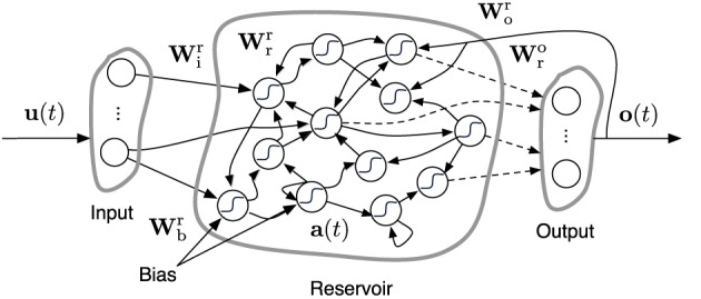
Keywords: MOSAIC; echo state networks; motor control; motor primitives; movement primitives; reservoir computing; robot control.

Figure 1

Illustration of MACOP which consists of an ensemble of controllers depicted in Figure 2. The desired (objective) and the current end-effector position are used as external inputs to each controller. The controller outputs are weighted by a scaling factor ζ_i and superimposed with each other such that the resulting joint-angles control the robot. The used ζ_i represent the responsibility of a controller and is determined by the measured joint-angles and end-effector position.

Figure 2

Schematic representation of a single controller. Model A and B are identical at every moment in time, but receive different input signals. The optional limiter limits the values x(t) to a desired range which, for example, represent imposed motor characteristics. Afterwards, the limited values $\tilde{x}(t)$ excite the plant (robot in this work). The signal $\tilde{x}(t-\delta )$ is the desired output which model A is trained to generate from the plant output, i.e., it learns the inverse model. This inverse model is then simultaneously employed as a controller to drive the plant (model B), which receives a desired future plant state y_d(t + δ) as input, instead of the actual one.

Figure 3

Description of an ESN. Dashed arrows are the connections which can be trained. Solid arrows are fixed. W^k_g is a matrix representing the connections from g to k, which stand for any of the letters r, i, o, b denoting reservoir, input, output, and bias, respectively. u(t), o(t) and a(t) represent the input, output, and reservoir states, respectively.

Figure 4

Illustration of a sudden change in desired joint-angle of the bottom joint (black dashed line) of the PUMA 500. The robot response is shown for this particular joint with different P-parameters, to illustrate the effect of a changed P value. By decreasing the P-parameter the dynamic transition time from one position to the other increases.

Figure 5

Top panel: the resulting end-effector trajectory generated by the robot arm for the rectangular target trajectory after convergence (RMSE < 1 mm for the full trajectory). The corresponding color of the dominant controller is shown. Bottom panel: the responsibility factors ζ_i(t) as a function of time.

Figure 6

Top panel: the resulting end-effector trajectory generated by the robot arm for the circular target trajectory after convergence. The corresponding color of the dominant controller is shown. The arrows indicate the direction of the trajectory. Bottom panel: the responsibility factors ζ_i(t) as a function of time.

Figure 7

Top panel: a part of the generated trajectory before the switch and after a jump, where the dominant controllers are represented by a corresponding color. The direction in which the trajectory is tracked is indicated by the arrows. Bottom panel: visualization of the generalization performance of the learned IK (circular training trajectory: dashed line) on a test grid. Color scale is the RMSE in m.

Figure 8

Illustration of the tracking performance of MACOP with 9 linear controllers after convergence. Top panel: the resulting trajectory, colored according to the dominant controller. The dashed line is the target. Bottom panel: the corresponding responsibilities as a function of time.

Figure 9

Effect of the number of controllers on the tracking performance of MACOP on the English alphabet trajectories. The mean, median, standard deviation, minimum and maximum values over 1300 experiments are shown for each controller configuration.

Figure 10

(A) Overview of the resulting trajectory with the “amarsi” target by using a single controller contribution. Each row shows the resulting end-effector trajectory of the robot arm. From left to right a part of the continuous writing is shown such that every letter of the word “amarsi” is presented. The coloring of the trajectory illustrates which controllers contribution is used (one for each row). The bottom row show the target trajectory, together with the actual generated trajectory. (B) The error of a single controller contribution (the black curves), plotted with their corresponding scaling factors (colored) as a function of time. The vertical scale of the error is provided on the left vertical axis, and that of the scaling on the right.

Figure 11

Comparison of the Z-coordinate of the generated trajectories for the shifted-squares objective. Shown are the desired Z-coordinate (black), and those generated by robots with P = 10 (blue), and P = 2 (red). The top panel is during the early parts of the training, and the bottom one after convergence. The abrupt change in the desired trajectory corresponds to the shift of the squares.

References

1. Bernstein N. A. (1967). The problem of interrelation of co-ordination and localization, in The Co-ordination and Regulation of Movements (New York, NY: Pergamon Press; ), 15–59
1. Bishop C. M., Nasrabadi N. M. (2006). Pattern Recognition and Machine Learning. Vol. 1 New York, NY: Springer
1. Bizzi E., Mussa-Ivaldi F. A., Giszter S. (1991). Computations underlying the execution of movement: a biological perspective. Science 253, 287–291 10.1126/science.1857964 - DOI - PubMed
1. Cheung V. C. K., d'Avella A., Tresch M. C., Bizzi E. (2005). Central and sensory contributions to the activation and organization of muscle synergies during natural motor behaviors. J. Neurosci. 25, 6419–6434 10.1523/JNEUROSCI.4904-04.2005 - DOI - PMC - PubMed
1. d'Avella A., Bizzi E. (2005). Shared and specific muscle synergies in natural motor behaviors. Proc. Natl. Acad. Sci. U.S.A. 102, 3076–3081 10.1073/pnas.0500199102 - DOI - PMC - PubMed