A network for scene processing in the macaque temporal lobe

Abstract

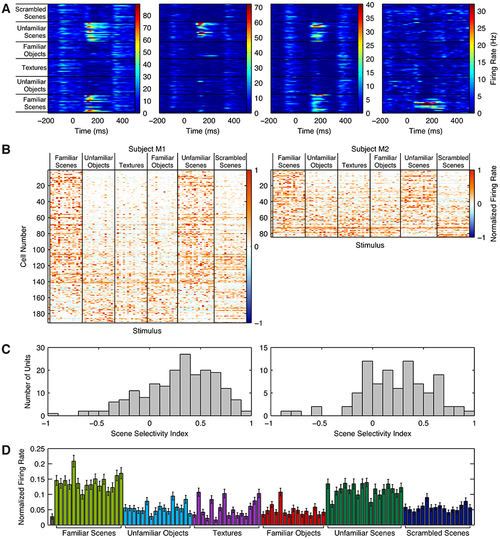
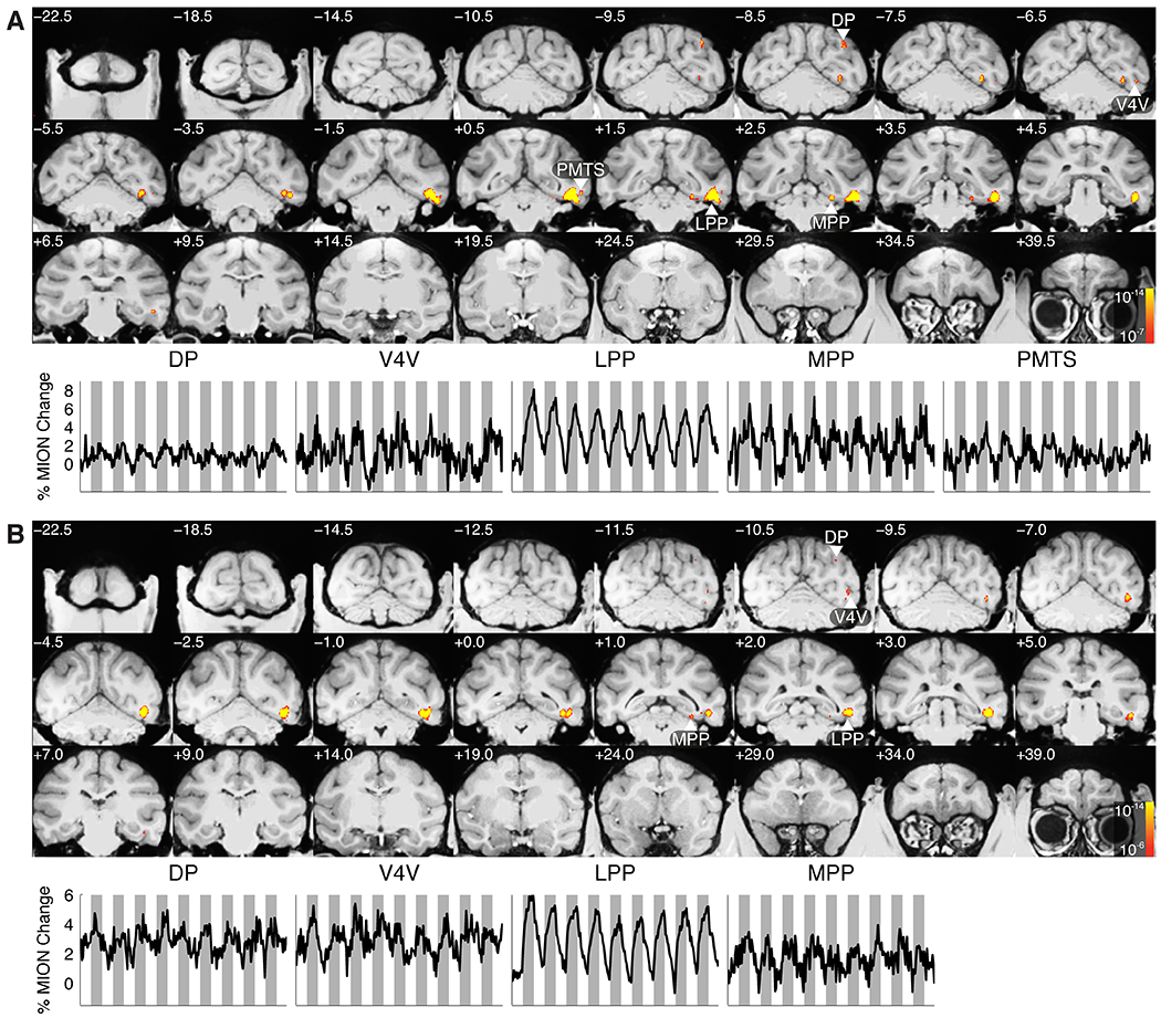
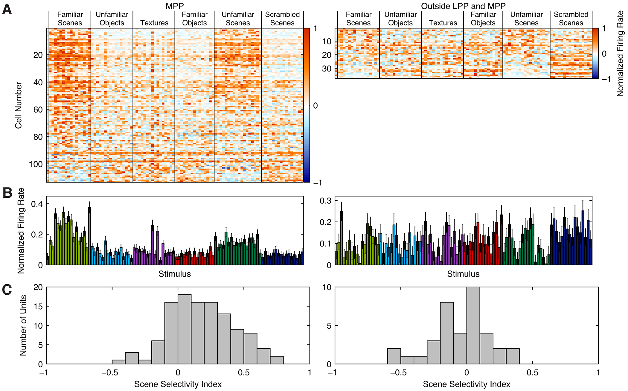
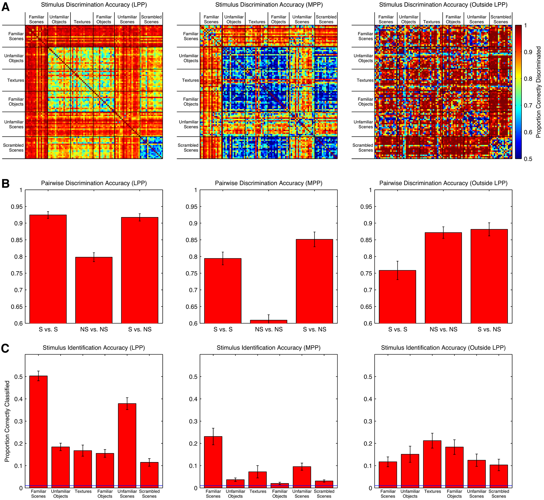
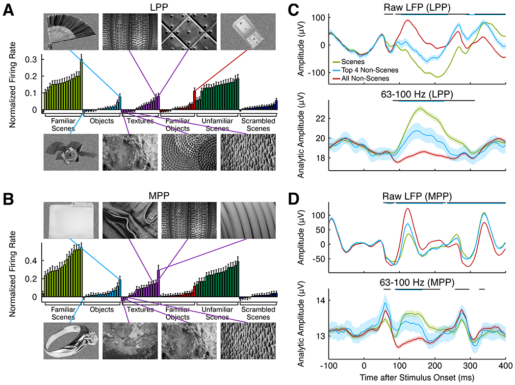
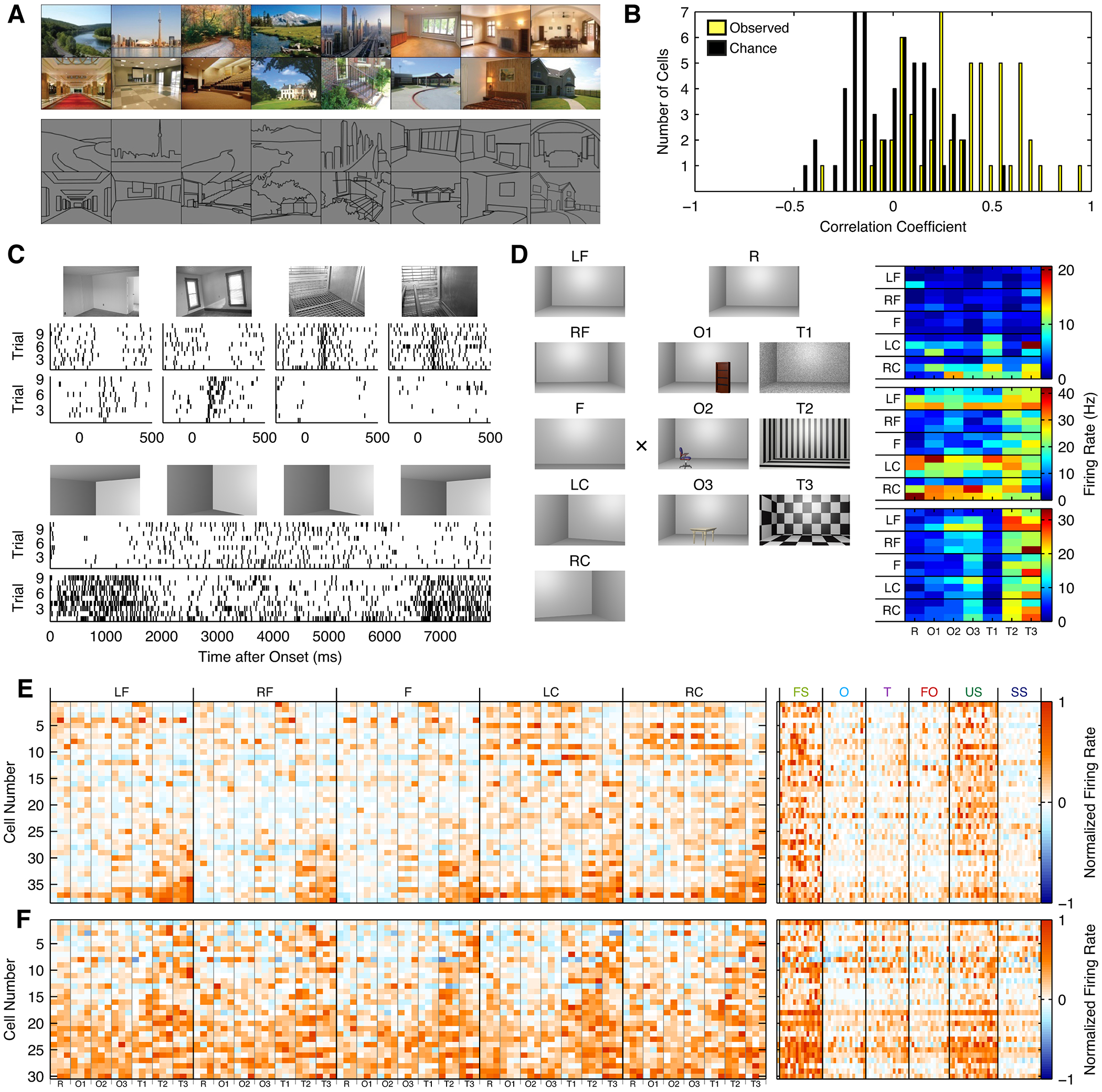
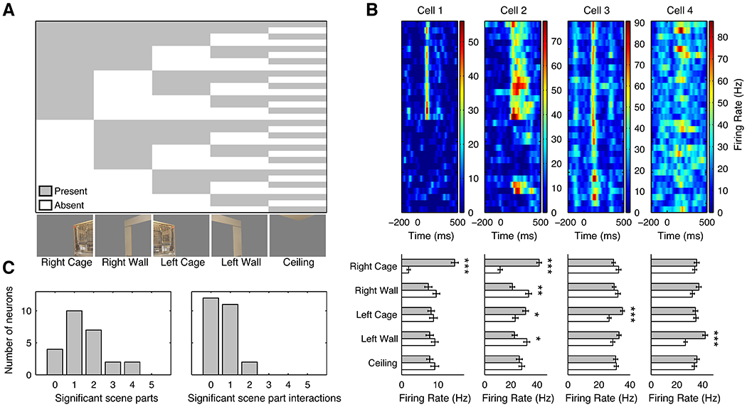
Spatial navigation is a complex process, but one that is essential for any mobile organism. We localized a region in the macaque occipitotemporal sulcus that responds preferentially to images of scenes. Single-unit recording revealed that this region, which we term the lateral place patch (LPP), contained a large concentration of scene-selective single units. These units were not modulated by spatial layout alone but were instead modulated by a combination of spatial and nonspatial factors, with individual units coding specific scene parts. We further demonstrate by microstimulation that LPP is connected with extrastriate visual areas V4V and DP and a scene-selective medial place patch in the parahippocampal gyrus, revealing a ventral network for visual scene processing in the macaque.

Figure 1:

A, Examples of stimuli shown. B, Coronal, sagittal, and horizontal slices indicating regions that exhibited a significantly greater response to scenes as compared to objects and textures in three monkeys. Fuchsia arrows indicate the location of the lateral place patch. Inset text indicates the AP coordinates of the coronal slice. C, Same as A, in a human subject. Fuchsia arrows indicate the location of the parahippocampal place area. D, Time course of the response to the localizer, averaged across the occipitotemporal place area of all monkeys in both hemispheres, and in the parahippocampal place area of a human subject. Regions of interest were defined on a separate set of runs from those from which the time courses were derived. Because blocks were shown in the same order on every run, with intervening blocks of scrambles to allow the hemodynamic signal to return to baseline, adaptation-related effects may confound comparison of the relative signal intensity among scene blocks. See also Figure S1.

Figure 2:

A, Response histograms for four example LPP single units. Cells 1 and 2 were recorded from M1; cells 3 and 4 were recorded from M2. B, Response profiles of visually responsive cells in LPP in M1 (left) and M2 (right), sorted by scene selectivity index. Each row represents one cell and each column one image. c, Histogram of scene selectivity indices for individual cells in M1 and M2. In both monkeys, the distribution was skewed toward positive values, indicating greater scene selectivity than would be expected by chance. D, Mean normalized response to each stimulus, averaged across all visually responsive cells. Scene stimuli evoked stronger activity than non-scene stimuli. Error bars are SEM. See also Figure S2.

Figure 3:

Areas showing significantly greater activation during microstimulation in the occipitotemporal place area as compared to baseline in subjects M1 (A) and M2 (B). Time courses for activated regions of interest are shown below the slice mosaic for each monkey. Shaded bars indicate time points during which microstimulation was active. Regions of interest were defined on one third of the data, while time courses were calculated from the remaining two thirds. See also Figure S3.

Figure 4:

Single unit responses to scenes and non-scenes in MPP (left) and a control region posterior to LPP (right). A, Response profiles of recorded cells. Each row represents one cell and each column one image. B, Mean normalized response to each stimulus, averaged across all visually responsive cells. Scene stimuli evoked stronger activity than non-scene stimuli in MPP, but not the control region posterior to LPP. Error bars are SEM. C, Histogram of scene selectivity indices.

Figure 5:

Performance of naïve Bayes classifiers in discriminating pairs of stimuli and identifying individual stimuli based on responses of 25 visually responsive single units in LPP (left), MPP (middle), and a control region posterior to LPP (right). A, Performance of classifier in distinguishing between pairs of stimuli. B, Average pairwise discrimination performance in each region for scenes versus scenes, non-scenes versus non-scenes, and scenes versus non-scenes. Chance performance is 50%. Error bars are SEM. C, Classifier accuracy in identifying individual stimuli from the full set of 98. Chance performance is 1%. Error bars are SEM.

Figure 6:

A and B, Mean normalized firing rate of visually responsive cells with scene selectivity index > ⅓ to each stimulus in the electrophysiology localizer in LPP (A) and MPP (B). Significant variance is visible in the magnitude of the mean response for non-scene stimuli. The four non-scene stimuli eliciting the strongest responses are shown above the graph; the four non-scene stimuli eliciting the weakest responses are shown below. C and D, Average LFP (top) and analytic amplitude in 63–100 Hz frequency band (bottom) to all scenes, top 4 non-scenes (shown to the left), and all non-scenes, averaged across 86 channels recorded from LPP (C) and 184 channels recorded from MPP (D). Error bars are 95% confidence intervals. Black strips at the top of each graph indicate significant differences between scenes and non-scenes; cyan strips indicate significant differences between the top and bottom four non-scenes (α = 0.001, t-test).

Figure 7:

A, Examples of scene photographs (top) and corresponding line drawings (bottom) used. B, Histogram of the average correlation between photographs of scenes and line drawings of the same scenes. C, Two cells showing selectivity for images of top and bottom room corners (one cell/row). The top group of rasters show these cells responding to indoor scene images. The bottom group show the same two cells as in responding to top and bottom corners of a synthetic stimulus consisting of a 3D-rendered sequence panning from top to bottom to top of an empty room. D, Left: parameterized synthetic room stimuli. LF = front left; RF = front right; F = front; LC = left corner; RC = right corner; R = empty rooms; O = object; T = texture. Right: Three example cells from M1 demonstrating an interaction between response for texture and spatial viewpoint in parameterized synthetic room stimuli. Object and texture are shown on the x-axis, while viewpoint and depth are shown on the y-axis. E and F, Left: Response of scene-selective cells from M1 to the parameterized room stimuli from b in LPP (e) and MPP (f), sorted by the first principal component. Right: responses of the same cells to the place localizer stimuli. See also Figure S6.

Figure 8:

A, Stimulus conditions. An image of two sets of cages was separated into the right (contralateral) cage, right wall, left (ipsilateral) cage, left wall, and ceiling. All 31 combinations of five scene parts were shown. B, Top, average responses of four example cells to each combination of scene parts. Bottom, average responses in the presence (green bars) or absence (white bars) of a given scene parts. * = p < 0.05, ** = p < 0.01, *** = p < 0.001. Cell 1 responded only to the right cage. Cell 2 responded strongly to the right cage and weakly to the left cage when presented alone. Its response was inhibited by the presence of the left and right walls. Cell 3 responded to all stimulus parts except for the ceiling, but fired more strongly when the left cage was present. Cell 4 responded to the left wall. C, Distributions of the number of scene parts (left) and the number of pairwise interactions (right) that exerted a significant influence on cell firing for the cage scene for 25 cells (p < 0.05, Holm-corrected).

References

1. Aguirre GK, and D’Esposito M (1999). Topographical disorientation: a synthesis and taxonomy. Brain 122, 1613. - PubMed
1. Blatt GJ, and Rosene DL (1998). Organization of direct hippocampal efferent projections to the cerebral cortex of the rhesus monkey: Projections from CA1, prosubiculum, and subiculum to the temporal lobe. J. Comp. Neurol 392, 92–114. - PubMed
1. Blatt GJ, Pandya DN, and Rosene DL (2003). Parcellation of cortical afferents to three distinct sectors in the parahippocampal gyrus of the rhesus monkey: An anatomical and neurophysiological study. J. Comp. Neurol 466, 161–179. - PubMed
1. Boussaoud D, Desimone R, and Ungerleider LG (1991). Visual topography of area TEO in the macaque. J. Comp. Neurol 306, 554–575. - PubMed
1. Buhrmester M, Kwang T, and Gosling SD (2011). Amazon’s Mechanical Turk: A new source of inexpensive, yet high-quality, data? Perspect. Psychol. Sci 6, 3–5. - PubMed
Publication types
LinkOut - more resources