. 2012 Jan 31:150:255-326.
doi: 10.1002/9781118197714.ch6.

Efficient and Unbiased Sampling of Biomolecular Systems in the Canonical Ensemble: A Review of Self-Guided Langevin Dynamics

Affiliations

Efficient and Unbiased Sampling of Biomolecular Systems in the Canonical Ensemble: A Review of Self-Guided Langevin Dynamics

Xiongwu Wu et al. Adv Chem Phys. .

Abstract

This review provides a comprehensive description of the self-guided Langevin dynamics (SGLD) and the self-guided molecular dynamics (SGMD) methods and their applications. Example systems are included to provide guidance on optimal application of these methods in simulation studies. SGMD/SGLD has enhanced ability to overcome energy barriers and accelerate rare events to affordable time scales. It has been demonstrated that with moderate parameters, SGLD can routinely cross energy barriers of 20 kT at a rate that molecular dynamics (MD) or Langevin dynamics (LD) crosses 10 kT barriers. The core of these methods is the use of local averages of forces and momenta in a direct manner that can preserve the canonical ensemble. The use of such local averages results in methods where low frequency motion "borrows" energy from high frequency degrees of freedom when a barrier is approached and then returns that excess energy after a barrier is crossed. This self-guiding effect also results in an accelerated diffusion to enhance conformational sampling efficiency. The resulting ensemble with SGLD deviates in a small way from the canonical ensemble, and that deviation can be corrected with either an on-the-fly or a post processing reweighting procedure that provides an excellent canonical ensemble for systems with a limited number of accelerated degrees of freedom. Since reweighting procedures are generally not size extensive, a newer method, SGLDfp, uses local averages of both momenta and forces to preserve the ensemble without reweighting. The SGLDfp approach is size extensive and can be used to accelerate low frequency motion in large systems, or in systems with explicit solvent where solvent diffusion is also to be enhanced. Since these methods are direct and straightforward, they can be used in conjunction with many other sampling methods or free energy methods by simply replacing the integration of degrees of freedom that are normally sampled by MD or LD.


Figures

Fig. 1
Fig. 1
(a) The example function, q(t) = sin(2πϖt), and its evolving averages at three local average times: ϖtL = 0.1, 1, and 10. (b) The evolving average of the example function as a function of the frequency. The envelope curves show the amplitude as a function of ϖtL. At small ϖtL, which corresponds to a low frequency, the amplitude is approaching 1, very similar to that of the example function, while at a large ϖtL, which corresponds to a high frequency, the amplitude approaches 0.
Fig. 1
Fig. 1
(a) The example function, q(t) = sin(2πϖt), and its evolving averages at three local average times: ϖtL = 0.1, 1, and 10. (b) The evolving average of the example function as a function of the frequency. The envelope curves show the amplitude as a function of ϖtL. At small ϖtL, which corresponds to a low frequency, the amplitude is approaching 1, very similar to that of the example function, while at a large ϖtL, which corresponds to a high frequency, the amplitude approaches 0.
Fig. 2
Fig. 2
The energy surface of the skewed double well potential. The potential is symmetric around the y–axis and rxz=x2+z2 is the distance to the y-axis.
Fig. 3
Fig. 3
(a)Temperature in y-coordinates; (b) temperature in rxz.
Fig. 3
Fig. 3
(a)Temperature in y-coordinates; (b) temperature in rxz.
Fig. 4
Fig. 4
(a) Average potential energies in y-coordinates; (b) average potential energies in x-z direction.
Fig. 4
Fig. 4
(a) Average potential energies in y-coordinates; (b) average potential energies in x-z direction.
Fig. 5
Fig. 5
The low frequency and high frequency temperatures at different local average time.
Fig. 6
Fig. 6
Trajectories the particle on the double well potential. (a) LD simulation; (b) SGLD simulation with λ=1. (c) SGLDfp simulation with λ=1. The collision frequency is 10/ps and temperature is 80 K.
Fig. 7
Fig. 7
Transitions of the particle on the double well potential in high temperature LD simulations and in SGLD or SGLDfp simulations. x-axis is T for the LD simulations and is the self-guiding temperature, Tsg, for the SGLD or SGLDfp simulations. The guiding factors are labeled in the plot and the temperature is 80 K for the SGLD or SGLDfp simulations. The collision frequency is 10/ps and the transition count starts with 1. The simulation length is 1000 ns.
Fig. 8
Fig. 8
Transitions of the particle on the skewed double well potential at different collision frequencies and temperatures. A guiding factor of λ=1 was used for all simulations. The transition count starts with 1. The simulation length is 1000 ns. The energy barrier heights from the y-average energies are (a) 5.56 kT at T=100 K; (b) 9.89 kT at T=60 K; and (c) 15.1 kT at T=40 K.
Fig. 9
Fig. 9
SGLD simulations of the double well system at different local averaging time, tL. Upper panel shows the self-guiding temperatures and lower panel shows the transitions crossing the energy barrier. The simulations are performed at T=100 K and are 1000ns in length.
Fig. 10
Fig. 10
The potential energy distributions of the double well system. (a) SGLD unweighted; (b) SGLD reweighted; (c) SGLDfp. The collision frequency is 10/ps and temperature is 80 K.
Fig. 11
Fig. 11
The y-coordinate distributions of the double well system. (a) SGLD unweighted; (b) SGLD reweighted; (c) SGLDfp. The collision frequency is 10/ps and temperature is 80 K.
Fig. 12
Fig. 12
Root-mean-square deviations of the SGLD and SGLDfp distributions from the LD distributions. The upper panel shows the deviations in the potential energy distributions (kcal/mol) from Fig. 10 and the lower panel shows the deviations in the y-distributions from Fig. 11.
Fig. 13
Fig. 13
Average potential energies vs. diffusion constants for the argon liquid in the LD simulations at different temperatures (as labeled) and in the SGLD simulations at different guiding factors (as labeled). The collision frequency is 1/ps. The SGLD simulations were performed at 100 K.
Fig. 14
Fig. 14
A conformation of an alanine dipeptide. Chemical bonds are shown as sticks. Oxygen and nitrogen atoms are shown as red and blue, respectively. Two backbone dihedral angles, ϕ and ψ, are marked by arrows.
Fig. 15
Fig. 15
ϕ-ψ dihedral angle distribution of the alanine dipeptide in the LD, SGLD, and SGLDfp simulations. The collision frequency is γ=10/ps and simulation temperature is 300 K. A guiding factor of λ=1 was used for both the SGLD and SGLDfp simulations.
Fig. 16
Fig. 16
Average energies against transition rates in high temperature LD, SGLD, and SGLDfp simulations. The simulation temperatures of the LD simulations, as well as the guiding factors and the self-guiding temperatures of the SGLD and SGLDfp simulations, are labeled beside their data points. The collision frequency is γ=10/ps for all simulations. The simulation temperature is 300 K for the SGLD and SGLDfp simulations.
Fig. 17
Fig. 17
The representative conformations of the six major clusters of the pentamer peptide. Backbone atoms are shown as thick sticks and sidechain heavy atoms are shown as thin sticks. Hydrogen atoms are not shown for clarity. Atoms are colored grey, blue, red for carbon, nitrogen, and oxygen, respectively.
Fig. 18
Fig. 18
Conformational distributions in the LD, SGLD, and SGLDfp simulations. Conformational distances from the center conformations of cluster 1 and 2 are used as x and y coordinates to show the distributions in two dimensions. All simulations are done with γ=1/ps and T=300 K. The guiding factor is λ=0.5 for SGLD and λ=1 for SGLDfp.
Fig. 19
Fig. 19
Conformational transitions between the clusters in the first 2000 ps of the LD, SGLD, and SGLDfp simulations. All simulations are done with γ=1/ps and T=300 K. The guiding factor is λ=0.5 for SGLD and λ=1 for SGLDfp.
Fig. 20
Fig. 20
Five major clusters identified from the trajectory obtained from the 2 ns SGMD simulation (Wu & Wang 2000) (upper row: clusters I, II, and III; lower row: clusters IV and V).
Fig. 21
Fig. 21
Snapshots of the peptide conformations obtained in the two 10 ns MD simulations (Wu & Wang 2001): (a) simulation started from a fully extended conformation; (b) simulation started from a complete helix conformation.
Fig. 22
Fig. 22
Major secondary structure clusters observed during the 10 ns SGMD simulation with λ = 0.4 (Wu & Wang 2001). Conformations are clustered on the basis of the number and location of helix segments in the peptide.
Fig. 23
Fig. 23
Reversible b-hairpin folding simulation with SGMD (Wu & Brooks 2004; Wu et al 2002). (a) A typical folded structure of the peptide obtained in the simulation (at 21,000 ps). For clarity, side chain hydrogens are not shown. The backbone atoms are shown as thick sticks and side chain atoms as thin sticks. Interstrand hydrogen bonds are marked by dashed lines. Atoms are colored red for oxygen, blue for nitrogen, white for hydrogen, and green for the rest. (b) NMR NOEs observed in the peptide aqueous solution2 (arrow bars between residues) and the average hydrogen pair distances (numbers in Å above NOE bars) in the β-hairpin structure obtained in our simulation. α, N, sc, and b represent the hydrogen atoms on α-carbon, amide nitrogen, side chain (β-carbon in our calculation), and backbone (amide nitrogen in our calculation). The thickness of the NOE bars represents the strength of the NOEs reported. Generally, NOEs are strong for hydrogen pair distances within 3 Å, medium between 3 and 4 Å, and week between 4 and 5 Å.
Fig 24
Fig 24
Combined SGLD with replica-exchange in protein folding simulation (Lee & Olson 2010). Free-energy landscapes at respective melting temperatures (ΔGfold = 0) of individual simulations method/starting structure/simulation data〉 in the coordinates of potential energy, U, and Cα rmsd to native: (a) MD-ReX/trans/50–100 ns (T = 351.3 K), (b) MD-ReX/native/50–100 ns (T = 354.6 K), (c) MD-ReX/native/150–200 ns (T = 348.2 K), (d) LD-ReX/trans/50–100 ns (T = 290.1 K), (e) LD-ReX/native/50–100 ns (T = 335.1 K), (f) LD-ReX/native/150–200 ns (T = 353.9 K), (g) SGLD-81 ReX/trans/50–100 ns (T = 311.2 K), (h) SGLD-ReX/native/50–100 ns (T = 331.5 K), and (i) SGLDReX/native/150–200 ns (T = 306.4 K).
Fig. 25
Fig. 25
Characterization of prion denatured state with SGLD simulations (Lee & Chang 2010). (A) The NMR structure of huPrP121–231 (PDB 1hjn [19]), (B) fully unfolded huPrP 121–230 at 600 K with the disulfide-bond shown in red, and (C) the simulated denatured structure of huPrP from the most populated cluster. The helical regions I, II and III defined based on the native structure are colored in red, blue and magentas, respectively.
Fig. 26
Fig. 26
Poisson-Boltzmann molecular dynamics simulation with the self-guiding force (Wen et al 2004; Wen & Luo 2004). Superposition of theoretical native states (gray) and native-like structures found in folding simulations (black): (a) BBA1; (b) villin headpiece.
Fig. 27
Fig. 27
Bak BH3 simulation results with SGMD (Yang et al 2004). Effects of mutation on the helical propensity from the 10-ns wild type and R5G and R5A sampling simulations.
Fig 28
Fig 28
Solvent equilibrated models for protein z-dependent protease inhibitor and its initial reactive complex with coagulation factor Xa (Chandrasekaran et al 2009).
Fig. 29
Fig. 29
Guest-host binding simulation with SGMD (Varady et al 2002). Starting Conformations for SGMD (SGMD #1 and #2) and Corresponding MD Simulations (MD #3 and #4). For clarity, only heavy atoms are shown. The six benzyl alcohol molecules are either all around the “rim” of the host (top) or four around the rim, one “below” and one “above” β-cyclodextrin (bottom).
Fig. 30
Fig. 30
Distance between the centers of the mass of guest and host molecules during MD and SGMD simulations (Varady et al 2002). For clarity, we plotted only the distances for guest molecules, which become tightly bound (within 3 Å) to the host molecule for longer than 30 ps during simulations.
Fig. 31
Fig. 31
Four major conformational clusters of G1 identified from an SGMD simulation in explicit water (Lung et al 2001). These clusters were identified using all 500 conformations recorded during the 500 ps SGMD simulation. The conformations in conformational cluster (A) were similar to the starting conformation, whereas the conformations in the other three clusters were substantially different from the starting conformation, and exhibited circular open-chain backbone conformations lacking evidence of intramolecular interactions.
Fig 32
Fig 32
SNase conformational reorganization from SGLD simulations (Damjanovic et al 2008b). The residues undergoing change in the secondary structure are shown in red. The substituted ionizable groups are shown in stick representation.
Fig. 33
Fig. 33
Crystal structure of the V66E variant of SNase (Damjanovic et al 2008a). (right) Snapshots from MD simulations representative of the straight (left) and the twisted (right) conformation of the Glu-66 side chain.
Figure 34
Figure 34
SGLD simulation of Conformational transitions induced by dephosphorylation in the NtrC protein (Damjanovic et al 2009). A) NMR structure of the inactive form of NtrCr. The key helix 4 is shown in black. B) NMR structure of the active form of NtrCr. C) Conformations of the key helix, 4: dark gray and white are the NMR structures of the phosphorylated and dephosphorylated forms, respectively. In blue is the average structure from the SGLD simulations of the phosphorylated protein. In green and red are the average structures from the SGLD simulations of the dephosphorylated protein with His-84 neutral and protonated, respectively.
Fig. 35
Fig. 35
SGLD study of conformational changes in a membrane transporter protein lactose permease (LacY)(Pendse et al 2010). Proton translocation to Glu269 and sugar binding trigger LacY conformational change from the inward-facing to the outward-facing state
Fig. 36
Fig. 36
Molecular dynamics simulations of the ionic complementary peptide EAK16-II on the hydrophobic HOPG surface (Sheng et al 2010a; 2010b). The adsorption and initial assembly process of EAK16-II on the surface were revealed. Hydrophobic alanine residues are found to be energetically favorable when in contact with the HOPG surface. It is the hydrophobic interaction that drives the adsorption of the first peptide molecule.
Fig. 37
Fig. 37
Snapshots of the peptide EAK16-II on the HOPG surface (Sheng et al 2010a; 2010b). The carbon atoms consisting of the HOPG surface are colored in cyan, water molecules are colored in red. The two peptide molecules are displayed with vdW spheres, and the three residues alanine, glutamic acid, and lysine are colored in grey, red, and blue, respectively.
Fig. 38
Fig. 38
Crystallization of argon liquid observed in SGMD simulations (Wu & Wang 1999). Snapshots of the argon film system at T* = 0.501(60 K). (a) Initial liquid structure, (b) crystallized structure. A tetragonal periodic boundary condition with sides a = b = 28.53 Å along x- and y-axes and c = 57.06 Å along z-axis is applied to the system.
Fig. 39
Fig. 39
The potential energies of the super-cooled argon film system (T* = 0.501) during the crystallization simulations (Wu & Wang 1999). Simulations were T* = 0.501 and with tl = 0.2 ps and different values. The solid line represents the results from a conventional MD simulation. The dashed line, dotted line, and centered lines represent the results in the SGMD simulations with tl = 0.2 ps and = 0.02, 0.05, and 0.1, respectively.
Fig. 40
Fig. 40
Comparison of phase transition process in different simulations (Abe & Jitsukawa 2009). Coordination number with respect to the size of Cu precipitates in conventional MD, simulated-annealing MD (SAMD), and SGMD (λ=0.1, tL=0.2ps).

References

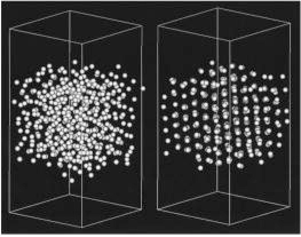
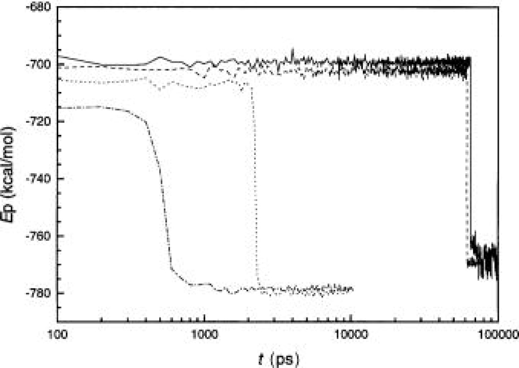
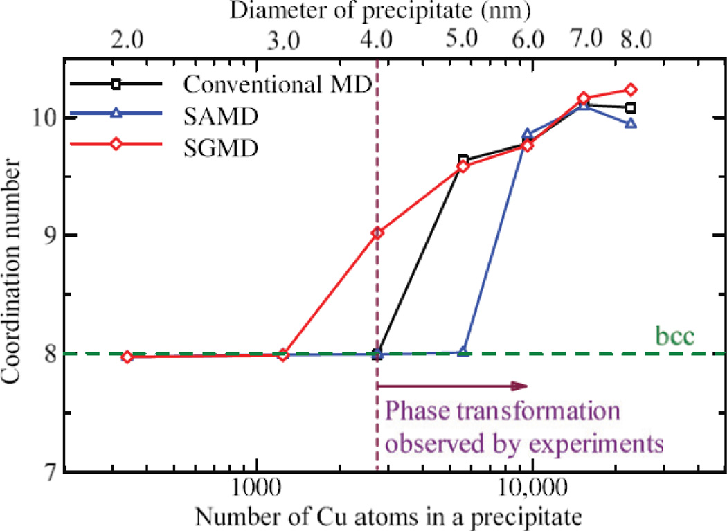
    1. Abe Y, Jitsukawa S. Phase transformation of Cu precipitate in Fe-Cu alloy studied using self-guided molecular dynamics. Philosophical Magazine Letters. 2009;89:535–543.
    1. Adcock SA, McCammon JA. Molecular dynamics: Survey of methods for simulating the activity of proteins. Chemical Reviews. 2006;106:1589–1615. - PMC - PubMed
    1. Allen MP, Tildesley DJ. Computer Simulations of Liquids. Oxford: Clarendon Press; 1987.
    1. Andricioaei I, Dinner AR, Karplus M. Self-guided enhanced sampling methods for thermodynamic averages. J. Chem. Phys. 2003;118:1074–1084.
    1. Beckers ML, Buydens LM, Pikkemaat JA, Altona C. Application of a genetic algorithm in the conformational analysis of methylene-acetal-linked thymine dimers in DNA: comparison with distance geometry calculations. J Biomol NMR. 1997;9:25–34. - PubMed

LinkOut - more resources