What is the primary cause of individual differences in contrast sensitivity?

Abstract

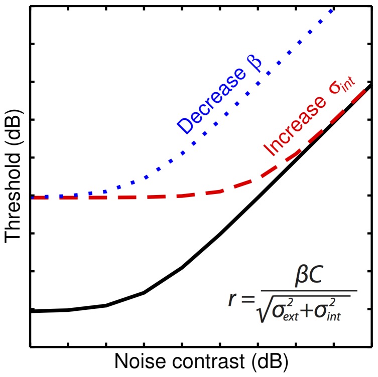
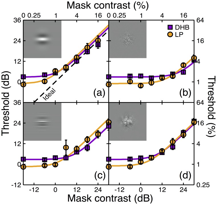
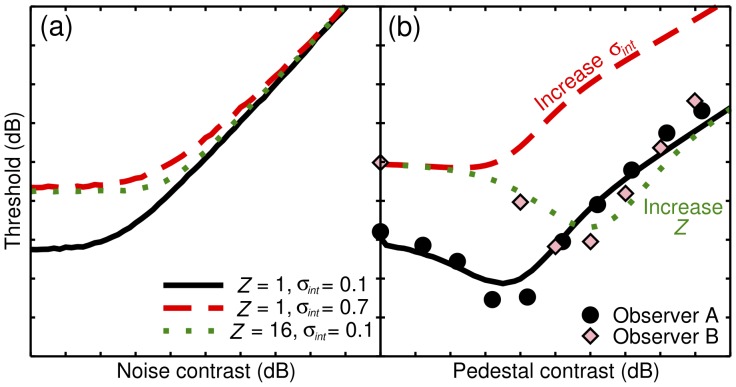
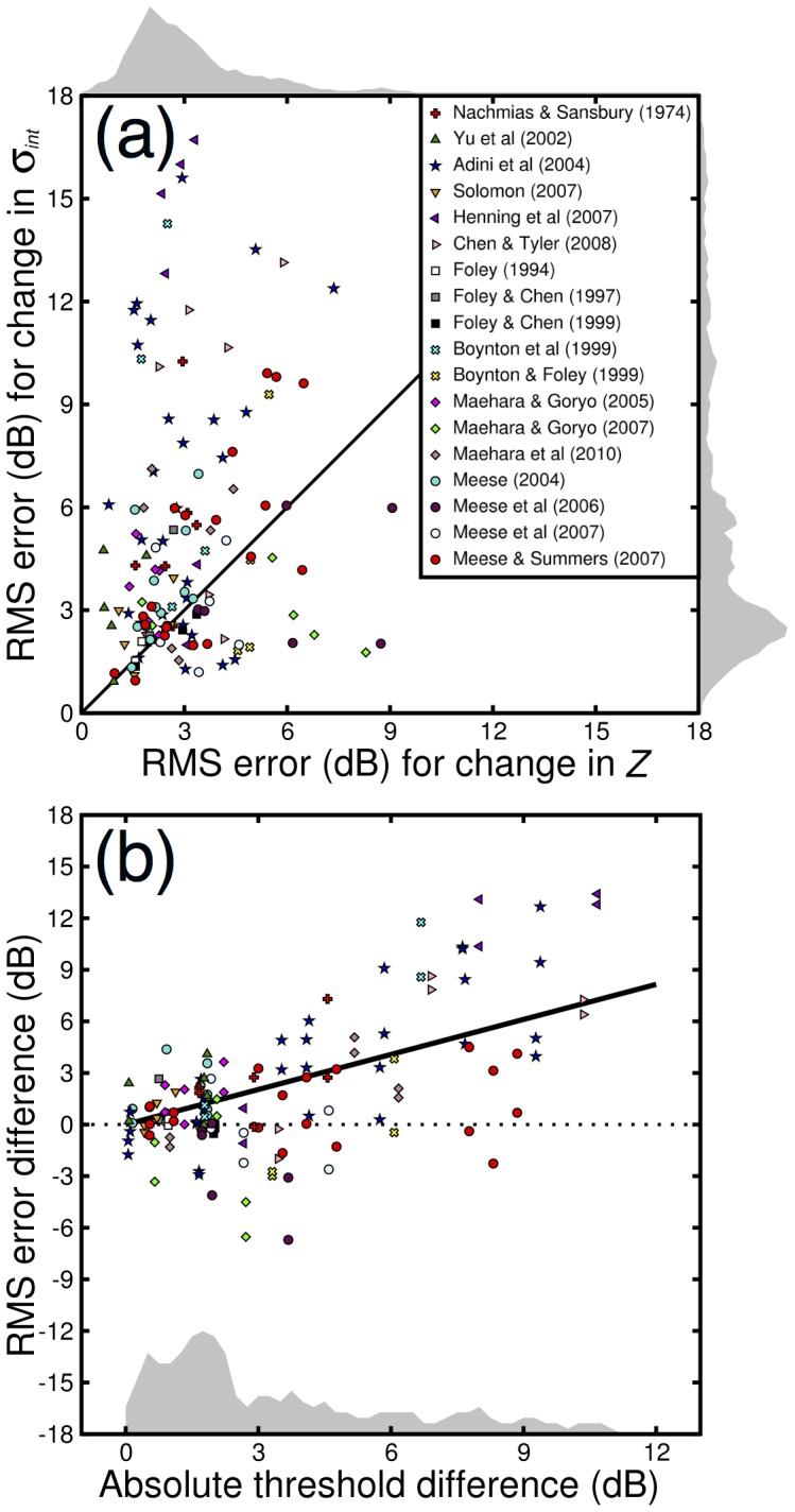
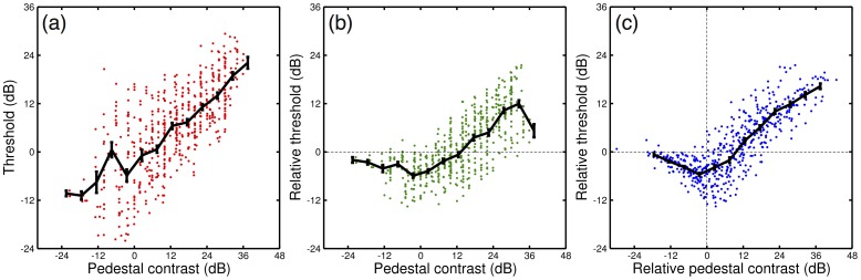
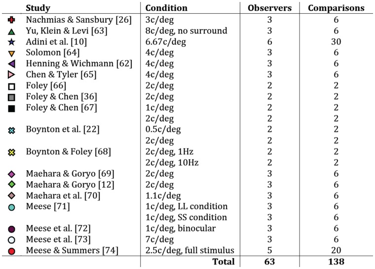
One of the primary objectives of early visual processing is the detection of luminance variations, often termed image contrast. Normal observers can differ in this ability by at least a factor of 4, yet this variation is typically overlooked, and has never been convincingly explained. This study uses two techniques to investigate the main source of individual variations in contrast sensitivity. First, a noise masking experiment assessed whether differences were due to the observer's internal noise, or the efficiency with which they extracted information from the stimulus. Second, contrast discrimination functions from 18 previous studies were compared (pairwise, within studies) using a computational model to determine whether differences were due to internal noise or the low level gain properties of contrast transduction. Taken together, the evidence points to differences in contrast gain as being responsible for the majority of individual variation across the normal population. This result is compared with related findings in attention and amblyopia.

Figure 1. Canonical noise masking functions showing the effect of changing model parameters.

The dashed and dotted curves show the effect of changing the level of internal noise (σ_int in equation 2– see Materials and Methods section) or the observer’s efficiency (β in equation 2), relative to the solid curve.

Figure 2. Noise masking functions for two observers and four varieties of external noise.

Insets to each panel show examples of the noise stimuli. (a) 0D noise, (b) 2D white noise, (c) 1D white noise, (d) 2D pink noise. The 0D noise had the same spatial waveform as the target. Error bars show standard deviations of a population of bootstrap resamples. The curves are fits of a noisy linear observer model detailed in the text, that had two free parameters per curve. The oblique dashed line in panel (a) gives the prediction of the ideal observer.

Figure 3. Behaviour of a nonlinear gain control model for noise masking (a) and contrast discrimination (b).

The data in (b) are replotted from Henning & Wichmann and are for observers NAL (circles) and GBH (diamonds). In both panels, green dotted curves show the effect of increasing the Z parameter of equation 1, and red dashed curves show the effect of increasing σ_int, relative to the solid curves.

Figure 4. Scatterplots showing RMS errors for fits to 138 pairs of dipper functions.

In (a), points above the oblique line indicate that changing σ_int produced a worse fit (larger error) than changing Z. In (b), the difference between the two errors is plotted against the absolute difference in detection threshold for each pair of dippers. Points above the dotted line correspond to points above the oblique line in panel (a). For pairs with the largest threshold differences (e.g. >6dB) almost all points favour the change in Z. The solid black line is the best fitting regression line, constrained to pass through [0,0], and has a slope of 0.68. The shaded histograms in each panel show the density of points. Since these exhibit positive skew, the data were log-transformed before performing statistical tests.

Figure 5. Summary of 63 dipper functions, plotted three ways.

Panel (a) shows the raw data from 18 studies (dots) and a binned average (black line, bin width of 6dB). Panel (b) shows the same data with the thresholds (y-axis) normalized to the baseline detection threshold (i.e. pedestal contrast of 0%) for each observer. Panel (c) shows the same data but with both axes normalized to the baseline detection threshold. Error bars show ±1SE of the mean for each bin.

Figure 6. Details of 18 studies that contained dipper functions used in the meta-analysis.

The number of pairwise comparisons is determined by n*(n-1), where n is the number of observers who completed a given condition.

References

1. Hubel DH, Wiesel TN (1959) Receptive fields of single neurones in the cat’s striate cortex. J Physiol 148: 574–591. - PMC - PubMed
1. Owsley C, Sekuler R, Siemsen D (1983) Contrast sensitivity throughout adulthood. Vision Res 23: 689–699. - PubMed
1. Dobkins KR, Gunther KL, Peterzell DH (2000) What covariance mechanisms underlie green/red equiluminance, luminance contrast sensitivity and chromatic (green/red) contrast sensitivity? Vision Res 40: 613–628. - PubMed
1. Peterzell DH, Teller DY (1996) Individual differences in contrast sensitivity functions: the lowest spatial frequency channels. Vision Res 36: 3077–3085. - PubMed
1. Schefrin BE, Tregear SJ, Harvey LO Jr, Werner JS (1999) Senescent changes in scotopic contrast sensitivity. Vision Res 39: 3728–3736. - PubMed
LinkOut - more resources