Equilibria of an epidemic game with piecewise linear social distancing cost

Abstract

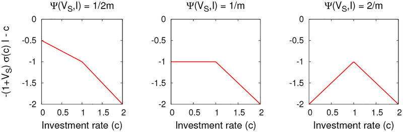
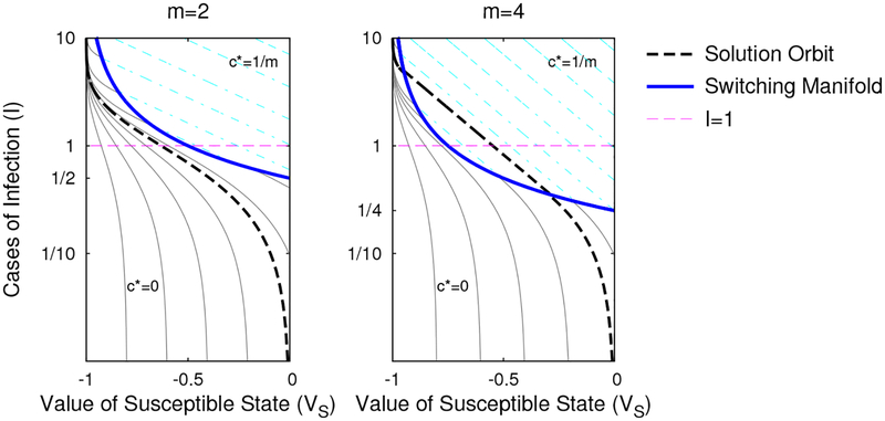
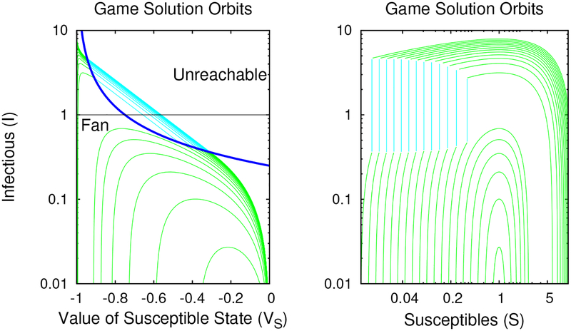
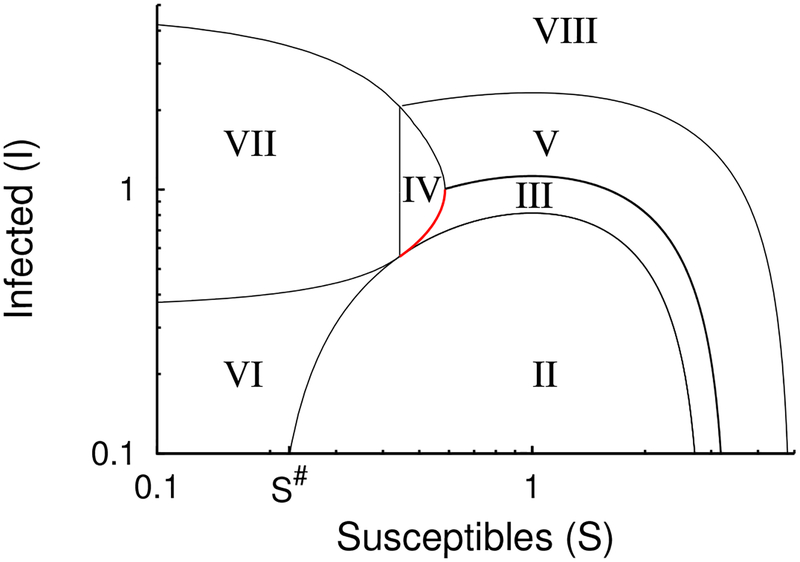
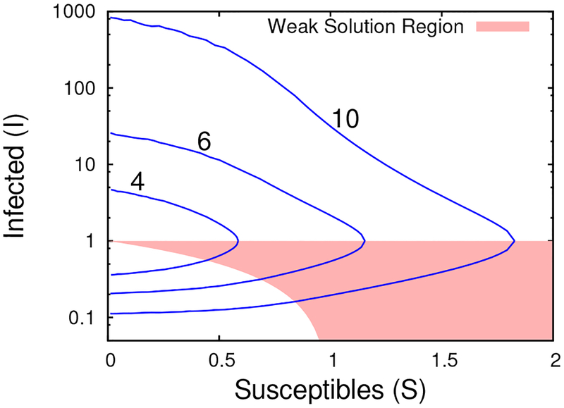
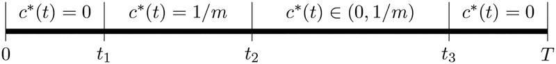
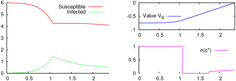
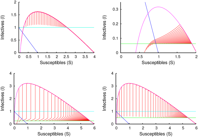
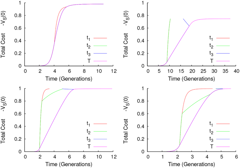
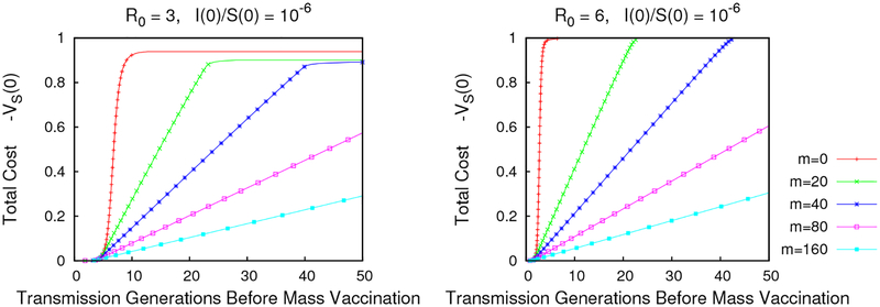
Around the world, infectious disease epidemics continue to threaten people's health. When epidemics strike, we often respond by changing our behaviors to reduce our risk of infection. This response is sometimes called "social distancing." Since behavior changes can be costly, we would like to know the optimal social distancing behavior. But the benefits of changes in behavior depend on the course of the epidemic, which itself depends on our behaviors. Differential population game theory provides a method for resolving this circular dependence. Here, I present the analysis of a special case of the differential SIR epidemic population game with social distancing when the relative infection rate is linear, but bounded below by zero. Equilibrium solutions are constructed in closed-form for an open-ended epidemic. Constructions are also provided for epidemics that are stopped by the deployment of a vaccination that becomes available a fixed-time after the start of the epidemic. This can be used to anticipate a window of opportunity during which mass vaccination can significantly reduce the cost of an epidemic.

Figure 1:

These 3 plots show how the objective −σ(c)I(1 + V_S) − c of our maximization in Eq. (1.2) depends on c for different choices of Ψ(V_S, I) when m = 1. When Ψ(V_S, I) < 1/m, the maximum occurs at c = 0. When Ψ(V_S, I) > 1/m, the maximum occurs at c = 1/m.

Figure 2:

Phase plane for our solution orbits to the infinite-horizon problem when S = 0 under Eq. (1.6) for efficiencies m = 2 (left) and m = 4 (right). The thick black dashed line is the solution matching the terminal conditions, and is a lower bound on all solutions reaching the terminal value in finite time. The thick blue solid line is the switching surface where c* jumps from c = 0 (gray solid) to c = 1/m (cyan dot-dashed). Along the switching surface, the flow is not differentiable but is continuous and unique. When the efficiency is above e ≈ 2.718 (right), the Nash equilibrium response always incorporates social distancing for sufficiently large I(0), independent of the terminal time. When the efficiency is below the threshold (left), then for every I(0) > 0, there are terminal times T sufficiently large that social distancing is never optimal. A log scale has been used on the I axis for illustration purposes.

Figure 3:

Regular equilibria trajectories in V_S × I phase space and S × I phase space for S(∞) ∈ [0, 1], I(∞) = V(∞) = 0, when σ(c) = max (1 − 4c, 0). The black curve from Fig. 2 corresponding to S = 0 is the least upper bound on the observed orbits; larger values of I for given V_S are unreachable. Orbits passing through the gap labelled “Fan” exist, but must be constructed using singular controls. The absence of intersecting trajectories in S × I space which would represent shocks and folds will be indicative of a unique Nash equilibrium for the infinite-horizon initial-value problem.

Figure 4:

When the efficiency m > e, the S × I phase plane is dissected into eight regions that are used in establishing the existence and uniqueness of an infinite-horizon Nash equilibrium for all initial conditions. In region II, orbits are the elementary solutions of the SIR model. Region III is part of a fan originating from the afferent manifold. Region IV is the opposite side of the fan, where c* = 1/m. Region V extends region IV, with c* = 0. Region VI contains orbits which hit the switching surface. Region VII extends Region VI with c* = 1/m. Region VIII extends Region VII with c* = 0. Every initial condition S(0), I(0) lies in one of these regions or on their boundaries, and has a unique initial value V_S(0) such that V_S(∞) = 0.

Figure 5:

Region of state-space where the differential inclusion specified by Eq. (1.3) and (1.6) may be multivalued when m = 5. If (S, I) falls inside this region and I(1 + V_S) = 1/m, the necessary condition only requires $C_s^{*}$ to be in the interval [0, 1/m]. Any singular equilibrium trajectory that tracks the switching surface must lie within the shaded region. Outside the shaded region, the necessary condition for $C_s^{*}$ is sufficient to uniquely determine integrated paths, even though $C_s^{*}$ itself is not everywhere uniquely determined. This applies for both infinite-horizon and finite-horizon analyses.

Figure 6:

Graph of the solutions S^#(m) of Eq. 4.13, depending on the slope m. There is no solution when m < e. Though the convergence rate is slow, lim_m→∞ S^#(m) = 1.

Figure 7:

Construction of curves where infinite-horizon equilibrium trajectories intersect the switching surface for different efficiencies m in S × I state space. For values of S(∞) < S^#(m) (red), the equilibrium passes directly through the switching surface, while for equilibria terminating with S(∞) = S^#(m), the equilibrium trajectory can either remain in the switching surface on the afferent manifold (blue) or exit on either side. The line I = 1 − S (black) is the break between these two behaviors. Note that while Fig. 6 shows S^#(m) increases slowly, this plot show that the intersection points with I = 1 − S increase more quickly. Curves for m = 3, 4, 6, 10, and 20.

Figure 8:

Construction of the complete set of equilibrium trajectories for the infinite horizon problem under Eq. (1.6) when m = 4. Green and cyan curves have c* = 0. Red and magenta curves have c* = ¼. the black curve at the center of the fan is the afferent manifold. The slight irregular spacing of the solutions is a consequence of sampling conditions chosen – a unique solution can be constructed to match any initial condition S(0), I(0).

Figure 9:

Boundaries of the regions of positive social distancing (c* > 0) for the equilibria of the infinite-horizon problem when σ(c) is given by Eq. (1.6) and the maximal efficiency of social distancing m ∈ {4, 6, 10}. The shaded region represents the portion of the state-space where singular controls are used to construct the equilibria.

Figure 10:

This is a timeline of equilibrium investment c*(t) between the start of the epidemic at time 0 and the termination of the epidemic at time T when universal vaccination occurs. To determine the equilibrium, we must calculate the times of each of the transition 0 ≤ t₁ ≤ t₂ ≤ t₃ ≤ T, along with the exact investment rate between times t₂ and t₃. In the case of S = 0, T = ∞, we always have t₂ = t₃, justifying the choice of notation in Section 3.

Figure 11:

An example time-series plot of the equilibrium trajectory to the finite-horizon problem calculated with S(0) = 6, I(0) = 0.01, m = 2, and T = 2.37. Panels show the state-variables S(t) and I(t) (left), along with the price of susceptibility V_S(t) (top right), and the relative contact rate σ(c*) under the equilibrium control c*(t) (bottom right). In this case, 0 < t₁ < t₂ < t₃ = T.

Figure 12:

Varieties of phase plane orbits for finite-time solutions for a range of initial expected values V (0) when I(0) ≈ 0. All numerical evidence indicates that final time T increases as the initial cost increases, which would imply uniqueness. Parameter values: S(0) = 4, m = 1 (top left), S(0) = 2, m = 16 (top right), S(0) = 6, m = 4 (bottom left), S(0) = 6, m = 2 (bottom right).

Figure 13:

This presents plots of the strategy change-times t₁, t₂, t₃ and T for the finite-time problem as the total cost V_S(0) varies when ${\mathcal{R}}_0=4$, m = 1 (top left), ${\mathcal{R}}_0=2$, m = 16 (top right), ${\mathcal{R}}_0=6$, m = 4 (bottom left), or ${\mathcal{R}}_0=6$, m = 2 (bottom right). Total distancing (t₁ ≠ t₂) is only used when vaccine deployment is very late. For faster deployment, Nash equilibrium makes use of managed distancing, where risks are perfectly balanced. For much of the range, the cost grows linearly with increases in delivery time. Conjecture 2 is supported by the observation that the T-curves appear to specify bijections between V_S(0) and the terminal time.

Figure 14:

Windows of Opportunity for Vaccination. Plots of how the net expected loss per individual depends on the amount of time until mass vaccination when (left) ${\mathcal{R}}_0=3$ and (right) ${\mathcal{R}}_0=6$. The windows are much longer than those found by Reluga (2010) for similar parameter values but σ = 1/(1 + mc), suggesting that equilibrium behaviors are sensitive to the shape of the tails of σ.

References

1. Arrow KJ and Kurz M (1970). Public Investment, the Rate of Return, and Optimal Fiscal Policy. Baltimore, MD: Johns Hopkins Press.
1. Auld M (2003). Choices, beliefs, and infectious disease dynamics. Journal of Health Economics 22, 361–377. - PubMed
1. Bressan A and Piccoli B (2007). Introduction to the Mathematical Theory of Control. American Institute of Mathematical Sciences.
1. Chen F (2012). A mathematical analysis of public avoidance behavior during epidemics using game theory. Journal of Theoretical Biology 302, 18–28. doi:10.1016/j.jtbi.2012.03.002. - DOI - PubMed
1. Chen F, Jiang M, Rabidoux S and Robinson S (2011). Public avoidance and epidemics: Insights from an economic model. Journal of Theoretical Biology 278, 107–119. doi:10.1016/j.jtbi.2011.03.007. - DOI - PubMed
Publication types
LinkOut - more resources