Toward a comprehensive framework for the spatiotemporal statistical analysis of longitudinal shape data

Abstract

This paper proposes an original approach for the statistical analysis of longitudinal shape data. The proposed method allows the characterization of typical growth patterns and subject-specific shape changes in repeated time-series observations of several subjects. This can be seen as the extension of usual longitudinal statistics of scalar measurements to high-dimensional shape or image data. The method is based on the estimation of continuous subject-specific growth trajectories and the comparison of such temporal shape changes across subjects. Differences between growth trajectories are decomposed into morphological deformations, which account for shape changes independent of the time, and time warps, which account for different rates of shape changes over time. Given a longitudinal shape data set, we estimate a mean growth scenario representative of the population, and the variations of this scenario both in terms of shape changes and in terms of change in growth speed. Then, intrinsic statistics are derived in the space of spatiotemporal deformations, which characterize the typical variations in shape and in growth speed within the studied population. They can be used to detect systematic developmental delays across subjects. In the context of neuroscience, we apply this method to analyze the differences in the growth of the hippocampus in children diagnosed with autism, developmental delays and in controls. Result suggest that group differences may be better characterized by a different speed of maturation rather than shape differences at a given age. In the context of anthropology, we assess the differences in the typical growth of the endocranium between chimpanzees and bonobos. We take advantage of this study to show the robustness of the method with respect to change of parameters and perturbation of the age estimates.

Keywords: growth; longitudinal data; shape regression; spatiotemporal registration; statistics; time warp.

Fig. 1

Synthetic example of a longitudinal data set with 3 subjects. Each subject has been observed a few times and at different time-points. The aim of the spatiotemporal variability analysis is to describe the variability of this population in two ways: the geometrical variability (there is a circle, a square and a triangle), and the variability in terms of change of dynamics of evolution (for instance, the square grows first at a faster rate than the circle and then slows down.)

Fig. 2

Illustration of the hypotheses underlying the subject- and time-specific approaches. In the subject-specific approach (left), one considers that one subject is “circle” and the other is “square”: the difference is described by a single function ϕ, which maps circles to squares. The evolution of the first subject is described by a function χ which maps a small circle to big circle. As a consequence, the evolution of the second subject is described by another function χ^ϕ which maps a small square to a big square. In the time-specific approach (right), one describes the evolution by a universal function χ, which tends to scale the shapes. At the first-time point, the difference between subjects is described by a function ϕ which maps the small circle to the small square. At a later time, the inter-subject variability has changed according to χ: now the difference between subjects is described by ϕ_t which maps a big circle to a big square.

Fig. 3

Subject- versus time-specific approach. In the subject-specific approach (left) the mean scenario averages the individual trajectories. The inter-subject variability is supposed to be constant over time. In the time-specific approach (right), every subject is supposed to follow the same mean scenario of evolution, up to a change of the initial conditions. The mean scenario describes how the inter-subject variability evolves over time.

Fig. 4

Shape regression of a set of five 2D profiles of hominid skulls (in red). The Australopithecus profile is chosen as the baseline S₀. The temporal regression computes a continuous flow of shapes S(t) (here in blue) such that the deforming shape matches the observations at the corresponding time-points. It is estimated by fitting a growth model, which assumes a diffeomorphic correspondence between the baseline and every stage of evolution (S(t) = χ_t (S₀)), with the diffeomorphism χ_t varying continuously in time.

Fig. 5

Illustrative pairwise registration: data preparation. The database is cut in two to compare the evolution {Homo habilis-erectus-neandertalensis} (red shapes) to the evolution {Homo erectus-sapiens sapiens} (green shapes). The later evolution is translated in time, so that both evolutions start at the same time. Then, one performs a shape regression of the source shapes (blue shapes). The spatiotemporal registration of this continuous source evolution to the target shapes is shown in Fig. 6 and 7.

Fig. 6

Illustrative pairwise registration: morphological deformation and time warp. Top row: The input data as prepared in Fig. 5 with the continuous source evolution (blue) superimposed with the target shapes (green). Middle row: The morphological deformation ϕ is applied to each frame of the source evolution. It shows that, independently of time, the skull is larger, rounder and the jaw less prominent during the later evolution relative to the earlier evolution. Bottom row: The time warp ψ is applied to the evolution of the second row. The blue shapes are moved along the time axis (as shown by dashed black lines), but they are not deformed. This change of the speed of evolution shows an acceleration of the later evolution relative to the earlier evolution. Taking this time warp into account enables a better alignment of the source to the target shapes than only the morphological deformation. Note that the morphological deformation and the time warp are estimated simultaneously, as the minimizers of a combined cost function.

Fig. 7

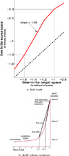
Illustrative pairwise registration: analysis of the time warp. Top: plot of the 1D time warp ψ(t) putting into correspondence the time-points of the target shapes with that of the source. The x = y line (dashed in black) would correspond to no dynamical change between source and target (ψ(t) = t). The slope indicates that the shape changes between target data occur 1.66 times faster than the changes in the source evolution, once morphological differences has been discarded. Right: the graph of the skull volume over the human evolution as found in the literature (source: www.bordalierinstitute.com). This curve shows that the increase in skull volume between Homo erectus and Homo sapiens sapiens was 1.62 times faster than between Homo habilis and Homo neandertalensis (ratio between the slope of the two straight lines). This value is compatible with the acceleration measured by the time warp: 1.66.

Fig. 8

Spatiotemporal atlas estimation given the two “subjects” in Fig. 5. On the middle row is shown the estimated mean scenario of evolution. The first frame of this scenario (far left) is the estimated template shape. Two upper rows represents the morphological deformation and then the time warp, which jointly maps the mean scenario to the shapes of the first subject (red shapes). Tow lower rows represents the spatiotemporal deformation of the mean scenario to the shapes of the second subject (green shapes). Black arrows indicate areas where the most important shape deformations occur.

Fig. 9

Spatiotemporal atlas estimation: template and time warp. (a) the template and its morphological deformation to the first subject (red) and the second subject (green). This corresponds to the far left frames in the second, third and fourth row in Fig. 8. (b) The graphs of the two time warps, mapping the subjects’ growth speed to that of the mean scenario. When the curve is above x = y axis, the subject’s evolution is in advance relative to the rate of shape changes given by the mean scenario. (c) Graph of the function: ${\psi }_1^{-1}○{\psi }_2$ (in blue), which maps the dynamics of the two subjects. The dashed red curve is the time warp given by the pairwise registration as shown in Fig. 7-a.

Fig. 10

Construction of 1D diffeomorphisms by integration of speed functions. In this illustration, we suppose the speed function to be constant (v independent of u): $\frac{\partial {\psi }_u(t)}{dt}=v({\psi }_u(t))$. Left: The speed profile v is set as the convolution of 3 constant momenta (β_i) with a Gaussian kernel with standard deviation λ_ψ = 4 (in red). The integration of the flow equation with the initial condition ψ₀(t) = t is shown in blue: the bold blue curve corresponds to the final diffeomorphism at u = 1, light blue curves correspond to ψ_1/6(t), ψ_1/3(t), ψ_1/2(t), ψ_2/3(t) and ψ_5/6(t). Right: Illustration of the numerical integration of the flow: ψ_un+1 (t) = ψ_un (t)+τv (ψ_un (t)). The speed profile in red is shown along the y-axis. One can show easily that this scheme produces only increasing function (invertible 1D function), when τ is chosen small enough.

Fig. 11

Illustrative scheme for the notations: x_p denotes a generic point of the source shape, x_p(t) = χ_t (x) the continuous evolution of the source point, (ψ_u)_{u∈[0, 1]} is a flow of 1D-diffeomorphism which moves the time-labels along the time-axis (in red), (ϕ_u)_{u∈[0, 1]} is a flow of 3D-diffeomorphism which moves the points of the source evolution (in magenta), independently at each time-point.

Fig. 12

Mean growth scenario of the hippocampus. Four significant frames are shown (lateral view). Color indicates the instantaneous speed of the surface deformation (best seen as a movie: see Online Resource 1)

Fig. 13

Evolution of the volume of the hippocampus. a- Volume evolution of the mean scenario. b-to d-: Volume of the mean scenario, after it has been registered to each subject (magenta curves). Black asterisks indicate the volume of the original data. Red, green and blue curves indicate the volume evolution given by the pairwise registration between each subject’s data pair. The autistic outlier corresponds to the decreasing red curve in b- (decrease of volume between the two observations of this subject)

Fig. 14

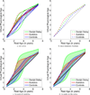
Estimated time warps from the hippocampus database. a- The monotonic curves indicates how the real age of each subject maps to the virtual physiological stage estimated in the mean growth scenario. When curves are above the x = y axis, the subject is in advance with respect to the mean scenario. The dashed red curve corresponds to the outlier. b- Intrinsic means of each group (also monotonic functions). c- Limits of the first mode of variation at ± one standard deviation. d- Same as c, but excluding the outlier. It shows that autistics tend to be in advance with respect to the control and that the developmental delays have a much greater variance than the other two groups.

Fig. 15

Estimated time warps from the amygdala database a- time warps for the 12 subjects, b- limits of the first mode of variation at ± 1 standard deviation for each group. Autistics and controls show the same evolution pattern, namely a reduction of speed with respect to the mean scenario (slope smaller than 1) and then a quick acceleration (slope greater than 1). This pattern for the autistics group seems to occur later than for the control group. The developmental delays presents also such pattern but at an arbitrary age. Mean and modes are computed as monotonic functions within the space of 1D diffeomorphisms.

Fig. 16

Temporal shape regression of endocast of the chimpanzees (top) and the bonobos (bottom) estimated from the original endocasts. In each species, the endocast seems to evolve from a spherical geometry at infancy to an ellipsoidal one at adulthood. However, the dynamics of such changes seem to differ for both species. The quite unrealistic evolution of the chimpanzee endocast at infancy is due to the small amount of data at this age (2). Here, only 6 stages of the growth are shown, although the estimated scenario is continuous. Best seen as movies: see Online Resource 2 (chimpanzees) and 3 (bonobos)

Fig. 17

From the continuous shape regression shown in Fig. 16, we deduce an estimation of the evolution of the endocast volume during growth. Mean and standard deviation of the volume of the original endocasts are superimposed. The intriguing decrease of volume of bonobos at sub-adulthood is not shown to be statistically significant. The unrealistic regression at infancy of chimpanzees is due to the very small number of samples at this age (2).

Fig. 18

Morphological part of the spatiotemporal registration between chimpanzees and bonobos growth scenarios. The morphological deformation maps the morphological space of the chimpanzees to that of the bonobos, independently of the age. It is applied here to the chimpanzees endocasts at old juvenility: endocasts from the chimpanzees growth scenario (top row), their deformation to the bonobos space (bottom row) with an intermediate stage of deformation (middle row). This shows that, on average, the endocast of a chimpanzee is more elongated and less round than the one of a bonobo. Note that the deformed endocasts do not match the ones of the bonobo growth at the same age, but at the age given by the correspondence graph shown in Fig. 19. Best seen as a movie: see Online Resource 4

Fig. 19

Time warp between chimpanzee and bonobo growth. It shows that the growth of the bonobos is in advance with respect to the chimpanzees at childhood and then that it drastically slows down during juvenility (almost linearly by a factor 0.24 between old-juvenility and sub-adulthood). This delay seems to decrease at adulthood. Dashed magenta lines indicate the limits of the 90% confidence interval estimated by bootstrap. Dashed cyan lines indicate the limits of the 90% variation intervals due to random age shifts.

Fig. 20

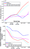
Effects of the spatiotemporal deformation on the evolution of the volume and the geometry of the endocasts. Top: Evolution of the endocast volume for the original growth scenarios of both species starting at childhood (in red and blue as in Fig. 17). Dashed cyan curve correspond to the volume of the chimpanzee growth scenario after the morphological deformation. Magenta curve is derived from the cyan curve by applying the time warp. The combination of the morphological deformation and the time warp approximate the volume evolution of the bonobos. Bottom: Same experiments but for the evolution of the ratio between the elongation in superior-inferior direction and that in the anteroposterior direction, which gives an indication of how the endocast deviates from a circular shape in the sagittal plane. The closer the ratio to 1, the “rounder” the endocast.

Fig. 21

Effect of the temporal scale λ_ψ on the registration accuracy. Value of the residual data term after registration for different values of the temporal scale λ_ψ (the other parameters being fixed to λ_ϕ = 10mm, σ_ϕ = 40, σ_ψ = 5, γ_ϕ = 10⁻⁵ and γ_ψ = 10⁻⁵). It indicates the optimal value of λ_ψ = 1 unit of time.

Fig. 22

Effect of the temporal scale λ_ψ on the time warp. If λ_ψ is too large, it cannot capture fast variations in the dynamics of growth of both species. If λ_ψ is too small, it costs more to capture the large-scaled variations. Optimal solution is for λ_ψ = 1 unit of time.

Fig. 23

Bootstrap confidence intervals due to resampling (top) and due to random age shifts (bottom). Left: Evolution of the endocranial volume given by the reference growth scenario (bold line) and its 90%-confidence interval estimated via a bootstrap procedure. Right: Discrepancy between the reference growth scenario and the ones estimated by bootstrap, measured as the current norm between the frames. 90% confidence interval is shown at every time-step. On average, the bootstrap makes the frames to vary in the space of currents within a neighborhood of radius 10% the norm of the reference frames.

References

1. Aljabar P, Bhatia K, Murgasova M, Hajnal J, Boardman J, Srinivasan L, Rutherford M, Dyet L, Edwards A, Rueckert D. Assessment of brain growth in early childhood using deformation-based morphometry. NeuroImage. 2008;39(1):348–358. - PubMed
1. Allassonnière S, Kuhn E. Stochastic algorithm for bayesian mixture effect template estimation. ESAIM Probability and Statistics. 2009 In Press.
1. Chandrashekara R, Rao A, Sanchez-Ortiz G, Mohiaddin RH, Rueckert D. Construction of a statistical model for cardiac motion analysis using nonrigid image registration. Information Processing in Medical Imaging, Springer, Lecture Notes in Computer Science. 2003;vol 2732:599–610. - PubMed
1. Courchesne E, Campbell K, Solso S. Brain growth across the life span in autism: Age-specific changes in anatomical pathology. Brain Research. 2011;1380:138–145. the Emerging Neuroscience of Autism Spectrum Disorders. - PMC - PubMed
1. de Craene M, Camara O, Bijnens BH, Frangi AF. Large diffeomorphic FFD registration for motion and strain quantification from 3D-US sequences. Proc. of Functional Imaging and Modeling of the Heart, Spinger, LNCS. 2009;vol 5528:437–446.
LinkOut - more resources